Code
pacman::p_load(olsrr, corrplot, ggpubr, sf, spdep, GWmodel, tmap, tidyverse, gtsummary, sfdep, onemapsgapi, stringr, SpatialML, devtools, tidymodels, kableExtra)Pandemic-induced supply chain constraints coinciding with the booming demand for flats have driven HDB resale prices up by 10.3% in 2022. For young couples deciding to buy a home to stay in, it seems nearly impossible to do so especially with the exorbitantly high price tags attached to flats recently.
This has caused many to think about what are the factors that affect the prices of HDB resale flats– some of which may be geographical in nature. For instance, some may pioritise of living near the local MRT, while others may focus on the location of schools within the vicinity of a flat.
In this take-home exercise, we will build a predictive model for the month of January and February 2023 in Singapore. The predictive models must be built by using by using conventional OLS method and GWR methods. Lastly, we will compare the performance of the conventional OLS method versus the geographical weighted methods.
The assignment submission is split into the following sections
pacman::p_load(olsrr, corrplot, ggpubr, sf, spdep, GWmodel, tmap, tidyverse, gtsummary, sfdep, onemapsgapi, stringr, SpatialML, devtools, tidymodels, kableExtra)The uses of each package installed can be found below:
kableExtra: an extension of kable, used for table customisation
onemapsgapi: used to query Singapore-specifif spatial data, alongside additional functionalities
httr: used to make API calls, such as GET requests
sf: used for importing, managing and processing geospatial data
spdep: used to create spatial weight matrix objects, global and local spatial autocorrelation statistics and related calculations
sfdep: builds on spdep to create sn sf and tidyverse friendly interface to the package
tidyverse: collection of R packages designed for data wrangling
stringr: provides a cohesive set of functions designed to make working with strings easily
olsrr: used for building least square regression models
corrplot + ggpubr: Used for multivariate data visualisation and analysis
GWmodel: provides a collection of localised spatial statistical methods such as summary statistic, principal components analysis, discriminant analysis and various forms of GW regression
gtsummary: provides an elegant and flexible way to create publication-ready analytical and summary tables using the R programming language
devtools: used for installing any R packages which is not available in RCRAN
SpatialML: allows for a geographically weighted random forest regression to include a function to find the optimal bandwidth
In this exercise, the collection of the coordinate data of singapore-specific places can tap on the database implemented by OneMapSg. 🏠
Referencing one of our senior Megan’s work, the steps to intialise this processes is as follows:
themesf <- st_as_sf(themetibble, coords=c("Lng", "Lat"), crs=4326)library(sf)
library(onemapsgapi)
token <- "your value"
search_themes(token, "searchval")
get_theme_status(token, "themename")
themetibble <- get_theme(token, "themename")
themesf <- st_as_sf(themetibble, coords=c("Lng", "Lat"), crs=4326)This token will expire on 2023-04-06 08:48:27# A tibble: 193 × 5
THEMENAME QUERY…¹ ICON CATEG…² THEME…³
<chr> <chr> <chr> <chr> <chr>
1 MCE KPE Speed Camera mce_kp… icon… Commun… LAND T…
2 Singapore Police Force Mobile Speed Cameras spf_msc Spee… Commun… SINGAP…
3 Liquor Control Zone(s) proclaimed under Liquor… liquor… Cres… Commun… SINGAP…
4 Singapore Police Force - 32nd ASEAN Summit Ist… as_ist… Cres… Commun… SINGAP…
5 Singapore Police Force - 32nd ASEAN Summit Ist… as_ist… Cres… Commun… SINGAP…
6 Inland Ash Scattering Gardens ias circ… Enviro… NATION…
7 CET Centres cetcen… WSQ.… Educat… SINGAP…
8 HDB Branches hdb_br… M090… Govern… HOUSIN…
9 Licensed premises for petroleum products custom… null null SINGAP…
10 NParks BBQ Pits nparks… null null NATION…
# … with 183 more rows, and abbreviated variable names ¹QUERYNAME, ²CATEGORY,
# ³THEME_OWNERWith that in mind, lets move on to data collection! 🙃
The following data would be used for the formation of our regression
# initialise a dataframe of our aspatial and geospatial dataset details
datasets <- data.frame(
  Type=c("Aspatial",
         "Geospatial",

         "Geospatial - Extracted",
         "Geospatial - Extracted",
         "Geospatial - Extracted",
         "Geospatial - Extracted",
         "Geospatial - Extracted",
         "Geospatial - Extracted",
         "Geospatial - Extracted",

         "Geospatial - Selfsourced",
         "Geospatial - Selfsourced",
         "Geospatial - Selfsourced",
         "Geospatial - Selfsourced",
         "Geospatial - Selfsourced"),

  Name=c("Resale Flat Prices",
         "Master Plan 2019 Subzone Boundary (Web)",

         "Childcare Services",
         "Eldercare Services",
         "Hawker Centres",
         "Kindergartens",
         "Parks",
         "Libraries",
         "Sport Facilities",

         "Bus Stop Locations Aug 2021",
         "MRT & LRT Locations Aug 2021",
         "Supermarkets",
         "Shopping Mall SVY21 Coordinates",
         "Primary School"),

  Format=c(".csv",
           ".shp",

           ".shp",
           ".shp",
           ".shp",
           ".shp",
           ".shp",
           ".shp",
           ".shp",

           ".shp",
           ".kml",
           ".shp",
           ".shp",
           ".csv"),

  Source=c("[data.gov.sg](https://data.gov.sg/dataset/resale-flat-prices)",
           "[data.gov.sg](https://data.gov.sg/dataset/master-plan-2014-subzone-boundary-web)",

           "[OneMap API](https://www.onemap.gov.sg/docs/)",
           "[OneMap API](https://www.onemap.gov.sg/docs/)",
           "[OneMap API](https://www.onemap.gov.sg/docs/)",
           "[OneMap API](https://www.onemap.gov.sg/docs/)",
           "[OneMap API](https://www.onemap.gov.sg/docs/)",
           "[OneMap API](https://www.onemap.gov.sg/docs/)",
           "[OneMap API](https://www.onemap.gov.sg/docs/)",

           "[datamall.lta](https://datamall.lta.gov.sg/content/datamall/en/search_datasets.html?searchText=bus%20stop)",
           "[data.gov](https://data.gov.sg/dataset/lta-mrt-station-exit)",
           "[Onemap.gov](https://www.onemap.gov.sg/main/v2/essentialamenities)",
           "[Valery Lim's Github](https://github.com/ValaryLim/Mall-Coordinates-Web-Scraper/blob/master/mall_coordinates_updated.csv)",
           "[data.gov](https://data.gov.sg/dataset/school-directory-and-information)")
  )

library(knitr)
library(kableExtra)
kable(datasets, caption="Datasets Used") %>%
kable_material("hover", latex_options="scale_down")| Type | Name | Format | Source |
|---|---|---|---|
| Aspatial | Resale Flat Prices | .csv | [data.gov.sg](https://data.gov.sg/dataset/resale-flat-prices) |
| Geospatial | Master Plan 2019 Subzone Boundary (Web) | .shp | [data.gov.sg](https://data.gov.sg/dataset/master-plan-2014-subzone-boundary-web) |
| Geospatial - Extracted | Childcare Services | .shp | [OneMap API](https://www.onemap.gov.sg/docs/) |
| Geospatial - Extracted | Eldercare Services | .shp | [OneMap API](https://www.onemap.gov.sg/docs/) |
| Geospatial - Extracted | Hawker Centres | .shp | [OneMap API](https://www.onemap.gov.sg/docs/) |
| Geospatial - Extracted | Kindergartens | .shp | [OneMap API](https://www.onemap.gov.sg/docs/) |
| Geospatial - Extracted | Parks | .shp | [OneMap API](https://www.onemap.gov.sg/docs/) |
| Geospatial - Extracted | Libraries | .shp | [OneMap API](https://www.onemap.gov.sg/docs/) |
| Geospatial - Extracted | Sport Facilities | .shp | [OneMap API](https://www.onemap.gov.sg/docs/) |
| Geospatial - Selfsourced | Bus Stop Locations Aug 2021 | .shp | [datamall.lta](https://datamall.lta.gov.sg/content/datamall/en/search_datasets.html?searchText=bus%20stop) |
| Geospatial - Selfsourced | MRT & LRT Locations Aug 2021 | .kml | [data.gov](https://data.gov.sg/dataset/lta-mrt-station-exit) |
| Geospatial - Selfsourced | Supermarkets | .shp | [Onemap.gov](https://www.onemap.gov.sg/main/v2/essentialamenities) |
| Geospatial - Selfsourced | Shopping Mall SVY21 Coordinates | .shp | [Valery Lim's Github](https://github.com/ValaryLim/Mall-Coordinates-Web-Scraper/blob/master/mall_coordinates_updated.csv) |
| Geospatial - Selfsourced | Primary School | .csv | [data.gov](https://data.gov.sg/dataset/school-directory-and-information) |
For the purpose of this take-home exercise, HDB Resale Flat Prices provided by Data.gov.sg should be used as the core data set.
The code chunk below reads the csv file into our R environment.
resale<-read_csv("data/aspatial/resale-flat-prices-based-on-registration-date-from-jan-2017-onwards.csv")
head(resale,5)The study should focus on either three-room, four-room or five-room flat and transaction period should be from 1st January 2021 to 31st December 2022. The test data should be January and February 2023 resale prices.
Therefore, we filter the dataset to include transactions occuring from Jan 2021 to Feb 2023.
# transaction period from 01-Jan-21 to 31-Feb-23
# 4-room flats
resale <- resale %>%
  filter(flat_type == "4 ROOM") %>%
filter(month >= "2021-01" & month <= "2022-12" | month >= "2023-01" & month <= "2023-02")resale$street_name <- gsub("ST\\.", "SAINT", resale$street_name)Notice that the data provided in the resale flat data does not include coordinates! We need to create our own geocoding function. With reference to our senior Megan’s work once again, these are the steps required in creating a geocoding function.
Combine the block and street name into an address
Pass the address as the searchVal in our query
Send the query to OneMapSG search Note: Since we don’t need all the address details, we can set getAddrDetails as ‘N’
Convert response (JSON object) to text
Save response in text form as a dataframe
We only need to retain the latitude and longitude for our output
library(httr)
library(rjson)
geocode <- function(block, streetname) {
  base_url <- "https://developers.onemap.sg/commonapi/search"
  address <- paste(block, streetname, sep = " ")
  query <- list("searchVal" = address,
                "returnGeom" = "Y",
                "getAddrDetails" = "N",
                "pageNum" = "1")

  res <- GET(base_url, query = query)
  restext<-content(res, as="text")

  output <- fromJSON(restext)  %>%
    as.data.frame %>%
    select(results.LATITUDE, results.LONGITUDE)

  return(output)
}With our function in place, we then create a loop to implement the geocoding function through our transaction data. ✌🏼
resale$LATITUDE <- 0
resale$LONGITUDE <- 0

for (i in 1:nrow(resale)){
  temp_output <- geocode(resale[i, 4], resale[i, 5])

  resale$LATITUDE[i] <- temp_output$results.LATITUDE
  resale$LONGITUDE[i] <- temp_output$results.LONGITUDE
}Especially given the extensive dataframe, this would take quite long to load! to avoid having to reload the output again, we save this as a RDS object 😵💫.
saveRDS(resale, file="resale", compress=FALSE)now we can read the resale file easily! 🤭
resale<-readRDS("resale")Our geospatial data can be split into several categories
| Base | Extracted | Sourced | |
|---|---|---|---|
| Description | geographical boundaries | Independent variable data extracted using OneMap API | Independent variable data extracted from the internet |
| Layer names |
|
childcare elder care hawker centre kindergartens parks libraries sport facilities |
|
Feel free to explore the codes we used to extract the data in the different panels below! 🤗
library(sf)
library(onemapsgapi)

# extracting eldercare data as an sf object into R
eldercare<-get_theme(token,"eldercare")
eldercare.sf <- st_as_sf(eldercare, coords=c("Lng", "Lat"), crs=4326)

# creating a saved sf object in data file for easy reference
st_write(obj = eldercare.sf,
         dsn = "data/geospatial/extracted",
         layer = "eldercare",
driver = "ESRI Shapefile")# extracting eldercare data as an sf object into R
hawkercentre<-get_theme(token,"hawkercentre")
hawkercentre.sf <- st_as_sf(hawkercentre, coords=c("Lng", "Lat"), crs=4326)
# creating a saved sf object in data file for easy reference
st_write(obj = hawkercentre.sf,
dsn = "data/geospatial/extracted",
layer = "hawkercentre",
driver = "ESRI Shapefile")# extracting childcare data as an sf object into R
childcare<-get_theme(token,"childcare")
childcare.sf <- st_as_sf(childcare, coords=c("Lng", "Lat"), crs=4326)
# creating a saved sf object in data file for easy reference
st_write(obj = childcare.sf,
dsn = "data/geospatial/extracted",
layer = "childcare",
driver = "ESRI Shapefile")# extracting kindergartens data as an sf object into R
kindergartens<-get_theme(token,"kindergartens")
kindergartens.sf <- st_as_sf(kindergartens, coords=c("Lng", "Lat"), crs=4326)
# creating a saved sf object in data file for easy reference
st_write(obj = kindergartens.sf,
dsn = "data/geospatial/extracted",
layer = "kindergartens",
driver = "ESRI Shapefile")# extracting parks data as an sf object into R
parks<-get_theme(token,"nationalparks")
parks.sf <- st_as_sf(parks, coords=c("Lng", "Lat"), crs=4326)
# creating a saved sf object in data file for easy reference
st_write(obj = parks.sf,
dsn = "data/geospatial/extracted",
layer = "parks",
driver = "ESRI Shapefile")# extracting library data as an sf object into R
library<-get_theme(token,"libraries")
library.sf <- st_as_sf(library, coords=c("Lng", "Lat"), crs=4326)
# creating a saved sf object in data file for easy reference
st_write(obj = library.sf,
dsn = "data/geospatial/extracted",
layer = "libraries",
driver = "ESRI Shapefile")Extracting and sports facility data:
sport<-get_theme(token,"sportsg_sport_facilities")

sport
When we browse the sports data, we see that the lat and lng columns are not configured in the way we expect it to be. In the Lng column, the longitude of the location is first placed followed by a “|” and then the latitude of the location. 🥲
Notice that the Lng and Lat are not in the format we want. We create a function to extract the Lng numbers from the string, using str_extract from the package stringr.
note the use of the following syntax
“\\d+” extracts one or more digits that occur before the | character
“\.?” matches the decimal point occuring in lng records
“\d*” matches any digits that come after the decimal point
lng.mutate<-function(df){
  df |>
    mutate(Lng=str_extract(Lng, "\\d+\\.?\\d*"))
}# extracting sports data as an sf object into R
sport<-get_theme(token,"sportsg_sport_facilities")
sport<-lng.mutate(sport)
sport.sf <- st_as_sf(sport, coords=c("Lng", "Lat"), crs=4326)
# creating a saved sf object in data file for easy reference
st_write(obj = sport.sf,
dsn = "data/geospatial/extracted",
layer = "sportsg_sport_facilities",
driver = "ESRI Shapefile")Bus stop data Extracted from: datamall.lta
Supermarkets extracted data from: Onemap.gov
Shopping mall data Extracted from: ValeryLim’s Github
since it is in a csv file, we convert it into a shape file and save it into our extracted data file in the code chunk below
mall.df<- read.csv("data/geospatial/sourced/mall_coordinates_updated.csv") |>
  select(latitude, longitude, name) |>
  dplyr::relocate(name)

mall.sf <- st_as_sf(mall.df, coords=c("longitude", "latitude"), crs=4326)

st_write(obj = mall.sf,
         dsn = "data/geospatial/sourced",
         layer = "shoppingmall",
driver = "ESRI Shapefile")Since only postal code and address data is given, we use the OneMapAPI in the code below to obtain coordinates of the schools.
primarysch.df<- read.csv("data/geospatial/sourced/general-information-of-schools.csv") |>
  dplyr::filter(mainlevel_code=="PRIMARY") |>
  dplyr::select(school_name, postal_code) |>
  dplyr::mutate(postal_code=ifelse(nchar(as.character(postal_code)) == 5,
                             paste0("0", as.character(postal_code)),
                             as.character(postal_code)))

#use onemap api
library(httr)
library(rjson)
geocode.data.gov <- function(postalcode) {
  base_url <- "https://developers.onemap.sg/commonapi/search"
  query <- list("searchVal" = postalcode,
                "returnGeom" = "Y",
                "getAddrDetails" = "N",
                "pageNum" = "1")

  res <- GET(base_url, query = query)
  restext<-content(res, as="text")

  output <- fromJSON(restext) |>
    as.data.frame() |>
    dplyr::select(results.LATITUDE, results.LONGITUDE)

  return(output)
}

#create loop to run data through
primarysch.df$LATITUDE <- 0
primarysch.df$LONGITUDE <- 0

for (i in 1:nrow(primarysch.df)){
  temp_output <- geocode.data.gov(primarysch.df[i, 2])

  primarysch.df$LATITUDE[i] <- temp_output$results.LATITUDE
  primarysch.df$LONGITUDE[i] <- temp_output$results.LONGITUDE
}

primarysch.sf <- st_as_sf(primarysch.df, coords=c("LONGITUDE", "LATITUDE"), crs=4326)

st_write(obj = primarysch.sf,
         dsn = "data/geospatial/sourced",
         layer = "primarysch",
driver = "ESRI Shapefile")Based on the rankings of this website, we take the first 10 schools
primarysch.sf <- st_read(dsn = "data/geospatial/sourced", layer = "primarysch")
goodprimarysch.sf <- primarysch.sf |>
  filter(school_name %in% c("NANYANG PRIMARY SCHOOL",
                            "TAO NAN SCHOOL",
                            "CANOSSA CATHOLIC PRIMARY SCHOOL",
                            "NAN HUA PRIMARY SCHOOL",
                            "ST. HILDA'S PRIMARY SCHOOL",
                            "HENRY PARK PRIMARY SCHOOL",
                            "ANGLO-CHINESE SCHOOL (PRIMARY)",
                            "RAFFLES GIRLS' PRIMARY SCHOOL",
                            "PEI HWA PRESBYTERIAN PRIMARY SCHOOL"
                            ))

st_write(obj = goodprimarysch.sf,
         dsn = "data/geospatial/sourced",
         layer = "goodprimarysch",
driver = "ESRI Shapefile")The data given to us is in “.kml” format, we convert it to an sf object.
mrt.sf<-st_read(dsn= "data/geospatial/sourced/lta-mrt-station-exit-kml.kml") |>
  st_zm()

st_write(obj = mrt.sf,
         dsn = "data/geospatial/sourced",
         layer = "mrt",
         driver = "ESRI Shapefile",
append = FALSE)mpsz.sf <- st_read(dsn = "data/geospatial/base", layer = "MPSZ-2019")Reading layer `MPSZ-2019' from data source
`/Users/pengyouyun/youyunpeng/IS415/Take-home_Ex/Take-home_Ex03/data/geospatial/base'
using driver `ESRI Shapefile'
Simple feature collection with 332 features and 6 fields
Geometry type: MULTIPOLYGON
Dimension: XYZ
Bounding box: xmin: 2667.538 ymin: 15748.72 xmax: 56396.44 ymax: 50256.33
z_range: zmin: 0 zmax: 0
Projected CRS: SVY21 / Singapore TMeldercare.sf <- st_read(dsn = "data/geospatial/extracted", layer = "eldercare")Reading layer `eldercare' from data source
`/Users/pengyouyun/youyunpeng/IS415/Take-home_Ex/Take-home_Ex03/data/geospatial/extracted'
using driver `ESRI Shapefile'
Simple feature collection with 133 features and 4 fields
Geometry type: POINT
Dimension: XY
Bounding box: xmin: 103.7119 ymin: 1.271472 xmax: 103.9561 ymax: 1.439561
Geodetic CRS: WGS 84hawkercentre.sf <- st_read(dsn = "data/geospatial/extracted", layer = "hawkercentre")Reading layer `hawkercentre' from data source
`/Users/pengyouyun/youyunpeng/IS415/Take-home_Ex/Take-home_Ex03/data/geospatial/extracted'
using driver `ESRI Shapefile'
Simple feature collection with 125 features and 18 fields
Geometry type: POINT
Dimension: XY
Bounding box: xmin: 103.6974 ymin: 1.272716 xmax: 103.9882 ymax: 1.449017
Geodetic CRS: WGS 84childcare.sf<- st_read(dsn = "data/geospatial/extracted", layer = "childcare")Reading layer `childcare' from data source
`/Users/pengyouyun/youyunpeng/IS415/Take-home_Ex/Take-home_Ex03/data/geospatial/extracted'
using driver `ESRI Shapefile'
Simple feature collection with 1925 features and 5 fields
Geometry type: POINT
Dimension: XY
Bounding box: xmin: 103.6878 ymin: 1.247759 xmax: 103.9897 ymax: 1.462134
Geodetic CRS: WGS 84kindergartens.sf<- st_read(dsn = "data/geospatial/extracted", layer = "kindergartens")Reading layer `kindergartens' from data source
`/Users/pengyouyun/youyunpeng/IS415/Take-home_Ex/Take-home_Ex03/data/geospatial/extracted'
using driver `ESRI Shapefile'
Simple feature collection with 448 features and 5 fields
Geometry type: POINT
Dimension: XY
Bounding box: xmin: 103.6887 ymin: 1.247759 xmax: 103.9717 ymax: 1.455452
Geodetic CRS: WGS 84parks.sf<- st_read(dsn = "data/geospatial/extracted", layer = "parks")Reading layer `parks' from data source
`/Users/pengyouyun/youyunpeng/IS415/Take-home_Ex/Take-home_Ex03/data/geospatial/extracted'
using driver `ESRI Shapefile'
Simple feature collection with 421 features and 2 fields
Geometry type: POINT
Dimension: XY
Bounding box: xmin: 103.6929 ymin: 1.214491 xmax: 104.0538 ymax: 1.462094
Geodetic CRS: WGS 84library.sf<- st_read(dsn = "data/geospatial/extracted", layer = "libraries")Reading layer `libraries' from data source
`/Users/pengyouyun/youyunpeng/IS415/Take-home_Ex/Take-home_Ex03/data/geospatial/extracted'
using driver `ESRI Shapefile'
Simple feature collection with 31 features and 13 fields
Geometry type: POINT
Dimension: XY
Bounding box: xmin: 103.7045 ymin: 1.263922 xmax: 103.9494 ymax: 1.448197
Geodetic CRS: WGS 84sport.sf<- st_read(dsn = "data/geospatial/extracted", layer = "sportsg_sport_facilities")Reading layer `sportsg_sport_facilities' from data source
`/Users/pengyouyun/youyunpeng/IS415/Take-home_Ex/Take-home_Ex03/data/geospatial/extracted'
using driver `ESRI Shapefile'
Simple feature collection with 35 features and 8 fields
Geometry type: POINT
Dimension: XY
Bounding box: xmin: 103.6937 ymin: 1.287668 xmax: 103.9524 ymax: 1.435755
Geodetic CRS: WGS 84busstop.sf <- st_read(dsn = "data/geospatial/sourced", layer = "BusStop")Reading layer `BusStop' from data source
`/Users/pengyouyun/youyunpeng/IS415/Take-home_Ex/Take-home_Ex03/data/geospatial/sourced'
using driver `ESRI Shapefile'
Simple feature collection with 5159 features and 3 fields
Geometry type: POINT
Dimension: XY
Bounding box: xmin: 3970.122 ymin: 26482.1 xmax: 48284.56 ymax: 52983.82
Projected CRS: SVY21shoppingmall.sf<-st_read(dsn = "data/geospatial/sourced", layer = "shoppingmall")Reading layer `shoppingmall' from data source
`/Users/pengyouyun/youyunpeng/IS415/Take-home_Ex/Take-home_Ex03/data/geospatial/sourced'
using driver `ESRI Shapefile'
Simple feature collection with 184 features and 1 field
Geometry type: POINT
Dimension: XY
Bounding box: xmin: 103.6784 ymin: 1.263797 xmax: 103.9897 ymax: 1.448227
Geodetic CRS: WGS 84supermarket.sf<-st_read(dsn = "data/geospatial/sourced", layer = "SUPERMARKETS")Reading layer `SUPERMARKETS' from data source
`/Users/pengyouyun/youyunpeng/IS415/Take-home_Ex/Take-home_Ex03/data/geospatial/sourced'
using driver `ESRI Shapefile'
Simple feature collection with 526 features and 8 fields
Geometry type: POINT
Dimension: XY
Bounding box: xmin: 4901.188 ymin: 25529.08 xmax: 46948.22 ymax: 49233.6
Projected CRS: SVY21mrt.sf<-st_read(dsn = "data/geospatial/sourced", layer = "mrt")Reading layer `mrt' from data source
`/Users/pengyouyun/youyunpeng/IS415/Take-home_Ex/Take-home_Ex03/data/geospatial/sourced'
using driver `ESRI Shapefile'
Simple feature collection with 474 features and 2 fields
Geometry type: POINT
Dimension: XY
Bounding box: xmin: 103.6368 ymin: 1.264972 xmax: 103.9893 ymax: 1.449157
Geodetic CRS: WGS 84primarysch.sf<-st_read(dsn = "data/geospatial/sourced", layer = "primarysch")Reading layer `primarysch' from data source
`/Users/pengyouyun/youyunpeng/IS415/Take-home_Ex/Take-home_Ex03/data/geospatial/sourced'
using driver `ESRI Shapefile'
Simple feature collection with 183 features and 2 fields
Geometry type: POINT
Dimension: XY
Bounding box: xmin: 103.6878 ymin: 1.274958 xmax: 103.9628 ymax: 1.456608
Geodetic CRS: WGS 84goodprimarysch.sf<-st_read(dsn = "data/geospatial/sourced", layer = "goodprimarysch")Reading layer `goodprimarysch' from data source
`/Users/pengyouyun/youyunpeng/IS415/Take-home_Ex/Take-home_Ex03/data/geospatial/sourced'
using driver `ESRI Shapefile'
Simple feature collection with 9 features and 2 fields
Geometry type: POINT
Dimension: XY
Bounding box: xmin: 103.7611 ymin: 1.305285 xmax: 103.937 ymax: 1.34968
Geodetic CRS: WGS 84For locational factor dataframes, we only need to know the name of the facility and its geometry column.
eldercare.sf<-select(eldercare.sf, 1)

hawkercentre.sf<-select(hawkercentre.sf, 1)

childcare.sf<-select(childcare.sf, 1)

parks.sf<-select(parks.sf, 1)

library.sf<-select(library.sf, 1)

sport.sf<-select(sport.sf, 1)

shoppingmall.sf<-select(shoppingmall.sf, 1)

busstop.sf<-select(busstop.sf, 1)

supermarket.sf<- select(supermarket.sf, 1)

primarysch.sf<-select(primarysch.sf, 1)

goodprimarysch.sf<-select(goodprimarysch.sf, 1)

mrt.sf<-select(mrt.sf, 1)length(which(st_is_valid(eldercare.sf) == FALSE))[1] 0length(which(st_is_valid(hawkercentre.sf) == FALSE))[1] 0length(which(st_is_valid(childcare.sf) == FALSE))[1] 0length(which(st_is_valid(kindergartens.sf) == FALSE))[1] 0length(which(st_is_valid(parks.sf) == FALSE))[1] 0length(which(st_is_valid(library.sf) == FALSE))[1] 0length(which(st_is_valid(sport.sf) == FALSE))[1] 0length(which(st_is_valid(busstop.sf) == FALSE))[1] 0length(which(st_is_valid(shoppingmall.sf) == FALSE))[1] 0length(which(st_is_valid(supermarket.sf) == FALSE))[1] 0length(which(st_is_valid(primarysch.sf) == FALSE))[1] 0length(which(st_is_valid(goodprimarysch.sf) == FALSE))[1] 0length(which(st_is_valid(mrt.sf) == FALSE))[1] 0length(which(st_is_valid(mpsz.sf) == FALSE))[1] 6We see that mpsz has 6 invalid geometries. Lets address them and check again
mpsz.sf <- st_make_valid(mpsz.sf)
length(which(st_is_valid(mpsz.sf) == FALSE))
[1] 0eldercare.sf[rowSums(is.na(eldercare.sf))!=0,]Simple feature collection with 0 features and 1 field
Bounding box: xmin: NA ymin: NA xmax: NA ymax: NA
Geodetic CRS: WGS 84
[1] NAME geometry
<0 rows> (or 0-length row.names)hawkercentre.sf[rowSums(is.na(hawkercentre.sf))!=0,]Simple feature collection with 0 features and 1 field
Bounding box: xmin: NA ymin: NA xmax: NA ymax: NA
Geodetic CRS: WGS 84
[1] NAME geometry
<0 rows> (or 0-length row.names)childcare.sf[rowSums(is.na(childcare.sf))!=0,]Simple feature collection with 0 features and 1 field
Bounding box: xmin: NA ymin: NA xmax: NA ymax: NA
Geodetic CRS: WGS 84
[1] NAME geometry
<0 rows> (or 0-length row.names)kindergartens.sf[rowSums(is.na(kindergartens.sf))!=0,]Simple feature collection with 0 features and 5 fields
Bounding box: xmin: NA ymin: NA xmax: NA ymax: NA
Geodetic CRS: WGS 84
[1] NAME DESCRIP ADDRESSP ADDRESSS ICON_NA geometry
<0 rows> (or 0-length row.names)parks.sf[rowSums(is.na(parks.sf))!=0,]Simple feature collection with 0 features and 1 field
Bounding box: xmin: NA ymin: NA xmax: NA ymax: NA
Geodetic CRS: WGS 84
[1] NAME geometry
<0 rows> (or 0-length row.names)library.sf[rowSums(is.na(library.sf))!=0,]Simple feature collection with 0 features and 1 field
Bounding box: xmin: NA ymin: NA xmax: NA ymax: NA
Geodetic CRS: WGS 84
[1] NAME geometry
<0 rows> (or 0-length row.names)sport.sf[rowSums(is.na(sport.sf))!=0,]Simple feature collection with 0 features and 1 field
Bounding box: xmin: NA ymin: NA xmax: NA ymax: NA
Geodetic CRS: WGS 84
[1] NAME geometry
<0 rows> (or 0-length row.names)busstop.sf[rowSums(is.na(busstop.sf))!=0,]Simple feature collection with 0 features and 1 field
Bounding box: xmin: NA ymin: NA xmax: NA ymax: NA
Projected CRS: SVY21
[1] BUS_STOP_N geometry
<0 rows> (or 0-length row.names)shoppingmall.sf[rowSums(is.na(shoppingmall.sf))!=0,]Simple feature collection with 0 features and 1 field
Bounding box: xmin: NA ymin: NA xmax: NA ymax: NA
Geodetic CRS: WGS 84
[1] name geometry
<0 rows> (or 0-length row.names)supermarket.sf[rowSums(is.na(supermarket.sf))!=0,]Simple feature collection with 0 features and 1 field
Bounding box: xmin: NA ymin: NA xmax: NA ymax: NA
Projected CRS: SVY21
[1] LIC_NAME geometry
<0 rows> (or 0-length row.names)primarysch.sf[rowSums(is.na(primarysch.sf))!=0,]Simple feature collection with 0 features and 1 field
Bounding box: xmin: NA ymin: NA xmax: NA ymax: NA
Geodetic CRS: WGS 84
[1] schl_nm geometry
<0 rows> (or 0-length row.names)goodprimarysch.sf[rowSums(is.na(goodprimarysch.sf))!=0,]Simple feature collection with 0 features and 1 field
Bounding box: xmin: NA ymin: NA xmax: NA ymax: NA
Geodetic CRS: WGS 84
[1] schl_nm geometry
<0 rows> (or 0-length row.names)mrt.sf[rowSums(is.na(mrt.sf))!=0,]Simple feature collection with 0 features and 1 field
Bounding box: xmin: NA ymin: NA xmax: NA ymax: NA
Geodetic CRS: WGS 84
[1] Name geometry
<0 rows> (or 0-length row.names)st_crs(mpsz.sf)Coordinate Reference System:
User input: SVY21 / Singapore TM
wkt:
PROJCRS["SVY21 / Singapore TM",
BASEGEOGCRS["SVY21",
DATUM["SVY21",
ELLIPSOID["WGS 84",6378137,298.257223563,
LENGTHUNIT["metre",1]]],
PRIMEM["Greenwich",0,
ANGLEUNIT["degree",0.0174532925199433]],
ID["EPSG",4757]],
CONVERSION["Singapore Transverse Mercator",
METHOD["Transverse Mercator",
ID["EPSG",9807]],
PARAMETER["Latitude of natural origin",1.36666666666667,
ANGLEUNIT["degree",0.0174532925199433],
ID["EPSG",8801]],
PARAMETER["Longitude of natural origin",103.833333333333,
ANGLEUNIT["degree",0.0174532925199433],
ID["EPSG",8802]],
PARAMETER["Scale factor at natural origin",1,
SCALEUNIT["unity",1],
ID["EPSG",8805]],
PARAMETER["False easting",28001.642,
LENGTHUNIT["metre",1],
ID["EPSG",8806]],
PARAMETER["False northing",38744.572,
LENGTHUNIT["metre",1],
ID["EPSG",8807]]],
CS[Cartesian,2],
AXIS["northing (N)",north,
ORDER[1],
LENGTHUNIT["metre",1]],
AXIS["easting (E)",east,
ORDER[2],
LENGTHUNIT["metre",1]],
USAGE[
SCOPE["Cadastre, engineering survey, topographic mapping."],
AREA["Singapore - onshore and offshore."],
BBOX[1.13,103.59,1.47,104.07]],
ID["EPSG",3414]]st_crs(eldercare.sf)Coordinate Reference System:
User input: WGS 84
wkt:
GEOGCRS["WGS 84",
DATUM["World Geodetic System 1984",
ELLIPSOID["WGS 84",6378137,298.257223563,
LENGTHUNIT["metre",1]]],
PRIMEM["Greenwich",0,
ANGLEUNIT["degree",0.0174532925199433]],
CS[ellipsoidal,2],
AXIS["latitude",north,
ORDER[1],
ANGLEUNIT["degree",0.0174532925199433]],
AXIS["longitude",east,
ORDER[2],
ANGLEUNIT["degree",0.0174532925199433]],
ID["EPSG",4326]]st_crs(hawkercentre.sf)Coordinate Reference System:
User input: WGS 84
wkt:
GEOGCRS["WGS 84",
DATUM["World Geodetic System 1984",
ELLIPSOID["WGS 84",6378137,298.257223563,
LENGTHUNIT["metre",1]]],
PRIMEM["Greenwich",0,
ANGLEUNIT["degree",0.0174532925199433]],
CS[ellipsoidal,2],
AXIS["latitude",north,
ORDER[1],
ANGLEUNIT["degree",0.0174532925199433]],
AXIS["longitude",east,
ORDER[2],
ANGLEUNIT["degree",0.0174532925199433]],
ID["EPSG",4326]]st_crs(childcare.sf)Coordinate Reference System:
User input: WGS 84
wkt:
GEOGCRS["WGS 84",
DATUM["World Geodetic System 1984",
ELLIPSOID["WGS 84",6378137,298.257223563,
LENGTHUNIT["metre",1]]],
PRIMEM["Greenwich",0,
ANGLEUNIT["degree",0.0174532925199433]],
CS[ellipsoidal,2],
AXIS["latitude",north,
ORDER[1],
ANGLEUNIT["degree",0.0174532925199433]],
AXIS["longitude",east,
ORDER[2],
ANGLEUNIT["degree",0.0174532925199433]],
ID["EPSG",4326]]st_crs(kindergartens.sf)Coordinate Reference System:
User input: WGS 84
wkt:
GEOGCRS["WGS 84",
DATUM["World Geodetic System 1984",
ELLIPSOID["WGS 84",6378137,298.257223563,
LENGTHUNIT["metre",1]]],
PRIMEM["Greenwich",0,
ANGLEUNIT["degree",0.0174532925199433]],
CS[ellipsoidal,2],
AXIS["latitude",north,
ORDER[1],
ANGLEUNIT["degree",0.0174532925199433]],
AXIS["longitude",east,
ORDER[2],
ANGLEUNIT["degree",0.0174532925199433]],
ID["EPSG",4326]]st_crs(parks.sf)Coordinate Reference System:
User input: WGS 84
wkt:
GEOGCRS["WGS 84",
DATUM["World Geodetic System 1984",
ELLIPSOID["WGS 84",6378137,298.257223563,
LENGTHUNIT["metre",1]]],
PRIMEM["Greenwich",0,
ANGLEUNIT["degree",0.0174532925199433]],
CS[ellipsoidal,2],
AXIS["latitude",north,
ORDER[1],
ANGLEUNIT["degree",0.0174532925199433]],
AXIS["longitude",east,
ORDER[2],
ANGLEUNIT["degree",0.0174532925199433]],
ID["EPSG",4326]]st_crs(library.sf)Coordinate Reference System:
User input: WGS 84
wkt:
GEOGCRS["WGS 84",
DATUM["World Geodetic System 1984",
ELLIPSOID["WGS 84",6378137,298.257223563,
LENGTHUNIT["metre",1]]],
PRIMEM["Greenwich",0,
ANGLEUNIT["degree",0.0174532925199433]],
CS[ellipsoidal,2],
AXIS["latitude",north,
ORDER[1],
ANGLEUNIT["degree",0.0174532925199433]],
AXIS["longitude",east,
ORDER[2],
ANGLEUNIT["degree",0.0174532925199433]],
ID["EPSG",4326]]st_crs(sport.sf)Coordinate Reference System:
User input: WGS 84
wkt:
GEOGCRS["WGS 84",
DATUM["World Geodetic System 1984",
ELLIPSOID["WGS 84",6378137,298.257223563,
LENGTHUNIT["metre",1]]],
PRIMEM["Greenwich",0,
ANGLEUNIT["degree",0.0174532925199433]],
CS[ellipsoidal,2],
AXIS["latitude",north,
ORDER[1],
ANGLEUNIT["degree",0.0174532925199433]],
AXIS["longitude",east,
ORDER[2],
ANGLEUNIT["degree",0.0174532925199433]],
ID["EPSG",4326]]st_crs(busstop.sf)Coordinate Reference System:
User input: SVY21
wkt:
PROJCRS["SVY21",
BASEGEOGCRS["WGS 84",
DATUM["World Geodetic System 1984",
ELLIPSOID["WGS 84",6378137,298.257223563,
LENGTHUNIT["metre",1]],
ID["EPSG",6326]],
PRIMEM["Greenwich",0,
ANGLEUNIT["Degree",0.0174532925199433]]],
CONVERSION["unnamed",
METHOD["Transverse Mercator",
ID["EPSG",9807]],
PARAMETER["Latitude of natural origin",1.36666666666667,
ANGLEUNIT["Degree",0.0174532925199433],
ID["EPSG",8801]],
PARAMETER["Longitude of natural origin",103.833333333333,
ANGLEUNIT["Degree",0.0174532925199433],
ID["EPSG",8802]],
PARAMETER["Scale factor at natural origin",1,
SCALEUNIT["unity",1],
ID["EPSG",8805]],
PARAMETER["False easting",28001.642,
LENGTHUNIT["metre",1],
ID["EPSG",8806]],
PARAMETER["False northing",38744.572,
LENGTHUNIT["metre",1],
ID["EPSG",8807]]],
CS[Cartesian,2],
AXIS["(E)",east,
ORDER[1],
LENGTHUNIT["metre",1,
ID["EPSG",9001]]],
AXIS["(N)",north,
ORDER[2],
LENGTHUNIT["metre",1,
ID["EPSG",9001]]]]st_crs(shoppingmall.sf)Coordinate Reference System:
User input: WGS 84
wkt:
GEOGCRS["WGS 84",
DATUM["World Geodetic System 1984",
ELLIPSOID["WGS 84",6378137,298.257223563,
LENGTHUNIT["metre",1]]],
PRIMEM["Greenwich",0,
ANGLEUNIT["degree",0.0174532925199433]],
CS[ellipsoidal,2],
AXIS["latitude",north,
ORDER[1],
ANGLEUNIT["degree",0.0174532925199433]],
AXIS["longitude",east,
ORDER[2],
ANGLEUNIT["degree",0.0174532925199433]],
ID["EPSG",4326]]st_crs(supermarket.sf)Coordinate Reference System:
User input: SVY21
wkt:
PROJCRS["SVY21",
BASEGEOGCRS["WGS 84",
DATUM["World Geodetic System 1984",
ELLIPSOID["WGS 84",6378137,298.257223563,
LENGTHUNIT["metre",1]],
ID["EPSG",6326]],
PRIMEM["Greenwich",0,
ANGLEUNIT["Degree",0.0174532925199433]]],
CONVERSION["unnamed",
METHOD["Transverse Mercator",
ID["EPSG",9807]],
PARAMETER["Latitude of natural origin",1.36666666666667,
ANGLEUNIT["Degree",0.0174532925199433],
ID["EPSG",8801]],
PARAMETER["Longitude of natural origin",103.833333333333,
ANGLEUNIT["Degree",0.0174532925199433],
ID["EPSG",8802]],
PARAMETER["Scale factor at natural origin",1,
SCALEUNIT["unity",1],
ID["EPSG",8805]],
PARAMETER["False easting",28001.642,
LENGTHUNIT["metre",1],
ID["EPSG",8806]],
PARAMETER["False northing",38744.572,
LENGTHUNIT["metre",1],
ID["EPSG",8807]]],
CS[Cartesian,2],
AXIS["(E)",east,
ORDER[1],
LENGTHUNIT["metre",1,
ID["EPSG",9001]]],
AXIS["(N)",north,
ORDER[2],
LENGTHUNIT["metre",1,
ID["EPSG",9001]]]]st_crs(primarysch.sf)Coordinate Reference System:
User input: WGS 84
wkt:
GEOGCRS["WGS 84",
DATUM["World Geodetic System 1984",
ELLIPSOID["WGS 84",6378137,298.257223563,
LENGTHUNIT["metre",1]]],
PRIMEM["Greenwich",0,
ANGLEUNIT["degree",0.0174532925199433]],
CS[ellipsoidal,2],
AXIS["latitude",north,
ORDER[1],
ANGLEUNIT["degree",0.0174532925199433]],
AXIS["longitude",east,
ORDER[2],
ANGLEUNIT["degree",0.0174532925199433]],
ID["EPSG",4326]]st_crs(goodprimarysch.sf)Coordinate Reference System:
User input: WGS 84
wkt:
GEOGCRS["WGS 84",
DATUM["World Geodetic System 1984",
ELLIPSOID["WGS 84",6378137,298.257223563,
LENGTHUNIT["metre",1]]],
PRIMEM["Greenwich",0,
ANGLEUNIT["degree",0.0174532925199433]],
CS[ellipsoidal,2],
AXIS["latitude",north,
ORDER[1],
ANGLEUNIT["degree",0.0174532925199433]],
AXIS["longitude",east,
ORDER[2],
ANGLEUNIT["degree",0.0174532925199433]],
ID["EPSG",4326]]st_crs(mrt.sf)Coordinate Reference System:
User input: WGS 84
wkt:
GEOGCRS["WGS 84",
DATUM["World Geodetic System 1984",
ELLIPSOID["WGS 84",6378137,298.257223563,
LENGTHUNIT["metre",1]]],
PRIMEM["Greenwich",0,
ANGLEUNIT["degree",0.0174532925199433]],
CS[ellipsoidal,2],
AXIS["latitude",north,
ORDER[1],
ANGLEUNIT["degree",0.0174532925199433]],
AXIS["longitude",east,
ORDER[2],
ANGLEUNIT["degree",0.0174532925199433]],
ID["EPSG",4326]]Note: our projected CRS should be SVY21 (EPSG code 3414). However, some of the extracted data sets are in WGS84, and others are in SVY21 with the incorrect EPSG code (EPSG 9001)
With the invalid geometries found earlier, we use the functions st_set_crs() and st_transform() to correct them.
#st_set_crs() assigns proper EPSG code
busstop.sf<-st_set_crs(busstop.sf, 3414)
Warning: st_crs<- : replacing crs does not reproject data; use st_transform for
thatsupermarket.sf<-st_set_crs(supermarket.sf, 3414)Warning: st_crs<- : replacing crs does not reproject data; use st_transform for
that#st_transform() changes CRS from one to another
eldercare.sf<-st_transform(eldercare.sf, crs=3414)
hawkercentre.sf<-st_transform(hawkercentre.sf, crs=3414)
childcare.sf<-st_transform(childcare.sf, crs=3414)
kindergartens.sf<-st_transform(kindergartens.sf, crs=3414)
parks.sf<-st_transform(parks.sf, crs=3414)
library.sf<-st_transform(library.sf, crs=3414)
sport.sf<-st_transform(sport.sf, crs=3414)
shoppingmall.sf<-st_transform(shoppingmall.sf, crs=3414)
primarysch.sf<-st_transform(primarysch.sf, crs=3414)
goodprimarysch.sf<-st_transform(goodprimarysch.sf, crs=3414)
mrt.sf<-st_transform(mrt.sf, crs=3414)Subsequently, we check again to make sure the data is in the proper CRS.
st_crs(mpsz.sf)Coordinate Reference System:
User input: SVY21 / Singapore TM
wkt:
PROJCRS["SVY21 / Singapore TM",
BASEGEOGCRS["SVY21",
DATUM["SVY21",
ELLIPSOID["WGS 84",6378137,298.257223563,
LENGTHUNIT["metre",1]]],
PRIMEM["Greenwich",0,
ANGLEUNIT["degree",0.0174532925199433]],
ID["EPSG",4757]],
CONVERSION["Singapore Transverse Mercator",
METHOD["Transverse Mercator",
ID["EPSG",9807]],
PARAMETER["Latitude of natural origin",1.36666666666667,
ANGLEUNIT["degree",0.0174532925199433],
ID["EPSG",8801]],
PARAMETER["Longitude of natural origin",103.833333333333,
ANGLEUNIT["degree",0.0174532925199433],
ID["EPSG",8802]],
PARAMETER["Scale factor at natural origin",1,
SCALEUNIT["unity",1],
ID["EPSG",8805]],
PARAMETER["False easting",28001.642,
LENGTHUNIT["metre",1],
ID["EPSG",8806]],
PARAMETER["False northing",38744.572,
LENGTHUNIT["metre",1],
ID["EPSG",8807]]],
CS[Cartesian,2],
AXIS["northing (N)",north,
ORDER[1],
LENGTHUNIT["metre",1]],
AXIS["easting (E)",east,
ORDER[2],
LENGTHUNIT["metre",1]],
USAGE[
SCOPE["Cadastre, engineering survey, topographic mapping."],
AREA["Singapore - onshore and offshore."],
BBOX[1.13,103.59,1.47,104.07]],
ID["EPSG",3414]]st_crs(eldercare.sf)Coordinate Reference System:
User input: EPSG:3414
wkt:
PROJCRS["SVY21 / Singapore TM",
BASEGEOGCRS["SVY21",
DATUM["SVY21",
ELLIPSOID["WGS 84",6378137,298.257223563,
LENGTHUNIT["metre",1]]],
PRIMEM["Greenwich",0,
ANGLEUNIT["degree",0.0174532925199433]],
ID["EPSG",4757]],
CONVERSION["Singapore Transverse Mercator",
METHOD["Transverse Mercator",
ID["EPSG",9807]],
PARAMETER["Latitude of natural origin",1.36666666666667,
ANGLEUNIT["degree",0.0174532925199433],
ID["EPSG",8801]],
PARAMETER["Longitude of natural origin",103.833333333333,
ANGLEUNIT["degree",0.0174532925199433],
ID["EPSG",8802]],
PARAMETER["Scale factor at natural origin",1,
SCALEUNIT["unity",1],
ID["EPSG",8805]],
PARAMETER["False easting",28001.642,
LENGTHUNIT["metre",1],
ID["EPSG",8806]],
PARAMETER["False northing",38744.572,
LENGTHUNIT["metre",1],
ID["EPSG",8807]]],
CS[Cartesian,2],
AXIS["northing (N)",north,
ORDER[1],
LENGTHUNIT["metre",1]],
AXIS["easting (E)",east,
ORDER[2],
LENGTHUNIT["metre",1]],
USAGE[
SCOPE["Cadastre, engineering survey, topographic mapping."],
AREA["Singapore - onshore and offshore."],
BBOX[1.13,103.59,1.47,104.07]],
ID["EPSG",3414]]st_crs(hawkercentre.sf)Coordinate Reference System:
User input: EPSG:3414
wkt:
PROJCRS["SVY21 / Singapore TM",
BASEGEOGCRS["SVY21",
DATUM["SVY21",
ELLIPSOID["WGS 84",6378137,298.257223563,
LENGTHUNIT["metre",1]]],
PRIMEM["Greenwich",0,
ANGLEUNIT["degree",0.0174532925199433]],
ID["EPSG",4757]],
CONVERSION["Singapore Transverse Mercator",
METHOD["Transverse Mercator",
ID["EPSG",9807]],
PARAMETER["Latitude of natural origin",1.36666666666667,
ANGLEUNIT["degree",0.0174532925199433],
ID["EPSG",8801]],
PARAMETER["Longitude of natural origin",103.833333333333,
ANGLEUNIT["degree",0.0174532925199433],
ID["EPSG",8802]],
PARAMETER["Scale factor at natural origin",1,
SCALEUNIT["unity",1],
ID["EPSG",8805]],
PARAMETER["False easting",28001.642,
LENGTHUNIT["metre",1],
ID["EPSG",8806]],
PARAMETER["False northing",38744.572,
LENGTHUNIT["metre",1],
ID["EPSG",8807]]],
CS[Cartesian,2],
AXIS["northing (N)",north,
ORDER[1],
LENGTHUNIT["metre",1]],
AXIS["easting (E)",east,
ORDER[2],
LENGTHUNIT["metre",1]],
USAGE[
SCOPE["Cadastre, engineering survey, topographic mapping."],
AREA["Singapore - onshore and offshore."],
BBOX[1.13,103.59,1.47,104.07]],
ID["EPSG",3414]]st_crs(childcare.sf)Coordinate Reference System:
User input: EPSG:3414
wkt:
PROJCRS["SVY21 / Singapore TM",
BASEGEOGCRS["SVY21",
DATUM["SVY21",
ELLIPSOID["WGS 84",6378137,298.257223563,
LENGTHUNIT["metre",1]]],
PRIMEM["Greenwich",0,
ANGLEUNIT["degree",0.0174532925199433]],
ID["EPSG",4757]],
CONVERSION["Singapore Transverse Mercator",
METHOD["Transverse Mercator",
ID["EPSG",9807]],
PARAMETER["Latitude of natural origin",1.36666666666667,
ANGLEUNIT["degree",0.0174532925199433],
ID["EPSG",8801]],
PARAMETER["Longitude of natural origin",103.833333333333,
ANGLEUNIT["degree",0.0174532925199433],
ID["EPSG",8802]],
PARAMETER["Scale factor at natural origin",1,
SCALEUNIT["unity",1],
ID["EPSG",8805]],
PARAMETER["False easting",28001.642,
LENGTHUNIT["metre",1],
ID["EPSG",8806]],
PARAMETER["False northing",38744.572,
LENGTHUNIT["metre",1],
ID["EPSG",8807]]],
CS[Cartesian,2],
AXIS["northing (N)",north,
ORDER[1],
LENGTHUNIT["metre",1]],
AXIS["easting (E)",east,
ORDER[2],
LENGTHUNIT["metre",1]],
USAGE[
SCOPE["Cadastre, engineering survey, topographic mapping."],
AREA["Singapore - onshore and offshore."],
BBOX[1.13,103.59,1.47,104.07]],
ID["EPSG",3414]]st_crs(kindergartens.sf)Coordinate Reference System:
User input: EPSG:3414
wkt:
PROJCRS["SVY21 / Singapore TM",
BASEGEOGCRS["SVY21",
DATUM["SVY21",
ELLIPSOID["WGS 84",6378137,298.257223563,
LENGTHUNIT["metre",1]]],
PRIMEM["Greenwich",0,
ANGLEUNIT["degree",0.0174532925199433]],
ID["EPSG",4757]],
CONVERSION["Singapore Transverse Mercator",
METHOD["Transverse Mercator",
ID["EPSG",9807]],
PARAMETER["Latitude of natural origin",1.36666666666667,
ANGLEUNIT["degree",0.0174532925199433],
ID["EPSG",8801]],
PARAMETER["Longitude of natural origin",103.833333333333,
ANGLEUNIT["degree",0.0174532925199433],
ID["EPSG",8802]],
PARAMETER["Scale factor at natural origin",1,
SCALEUNIT["unity",1],
ID["EPSG",8805]],
PARAMETER["False easting",28001.642,
LENGTHUNIT["metre",1],
ID["EPSG",8806]],
PARAMETER["False northing",38744.572,
LENGTHUNIT["metre",1],
ID["EPSG",8807]]],
CS[Cartesian,2],
AXIS["northing (N)",north,
ORDER[1],
LENGTHUNIT["metre",1]],
AXIS["easting (E)",east,
ORDER[2],
LENGTHUNIT["metre",1]],
USAGE[
SCOPE["Cadastre, engineering survey, topographic mapping."],
AREA["Singapore - onshore and offshore."],
BBOX[1.13,103.59,1.47,104.07]],
ID["EPSG",3414]]st_crs(parks.sf)Coordinate Reference System:
User input: EPSG:3414
wkt:
PROJCRS["SVY21 / Singapore TM",
BASEGEOGCRS["SVY21",
DATUM["SVY21",
ELLIPSOID["WGS 84",6378137,298.257223563,
LENGTHUNIT["metre",1]]],
PRIMEM["Greenwich",0,
ANGLEUNIT["degree",0.0174532925199433]],
ID["EPSG",4757]],
CONVERSION["Singapore Transverse Mercator",
METHOD["Transverse Mercator",
ID["EPSG",9807]],
PARAMETER["Latitude of natural origin",1.36666666666667,
ANGLEUNIT["degree",0.0174532925199433],
ID["EPSG",8801]],
PARAMETER["Longitude of natural origin",103.833333333333,
ANGLEUNIT["degree",0.0174532925199433],
ID["EPSG",8802]],
PARAMETER["Scale factor at natural origin",1,
SCALEUNIT["unity",1],
ID["EPSG",8805]],
PARAMETER["False easting",28001.642,
LENGTHUNIT["metre",1],
ID["EPSG",8806]],
PARAMETER["False northing",38744.572,
LENGTHUNIT["metre",1],
ID["EPSG",8807]]],
CS[Cartesian,2],
AXIS["northing (N)",north,
ORDER[1],
LENGTHUNIT["metre",1]],
AXIS["easting (E)",east,
ORDER[2],
LENGTHUNIT["metre",1]],
USAGE[
SCOPE["Cadastre, engineering survey, topographic mapping."],
AREA["Singapore - onshore and offshore."],
BBOX[1.13,103.59,1.47,104.07]],
ID["EPSG",3414]]st_crs(library.sf)Coordinate Reference System:
User input: EPSG:3414
wkt:
PROJCRS["SVY21 / Singapore TM",
BASEGEOGCRS["SVY21",
DATUM["SVY21",
ELLIPSOID["WGS 84",6378137,298.257223563,
LENGTHUNIT["metre",1]]],
PRIMEM["Greenwich",0,
ANGLEUNIT["degree",0.0174532925199433]],
ID["EPSG",4757]],
CONVERSION["Singapore Transverse Mercator",
METHOD["Transverse Mercator",
ID["EPSG",9807]],
PARAMETER["Latitude of natural origin",1.36666666666667,
ANGLEUNIT["degree",0.0174532925199433],
ID["EPSG",8801]],
PARAMETER["Longitude of natural origin",103.833333333333,
ANGLEUNIT["degree",0.0174532925199433],
ID["EPSG",8802]],
PARAMETER["Scale factor at natural origin",1,
SCALEUNIT["unity",1],
ID["EPSG",8805]],
PARAMETER["False easting",28001.642,
LENGTHUNIT["metre",1],
ID["EPSG",8806]],
PARAMETER["False northing",38744.572,
LENGTHUNIT["metre",1],
ID["EPSG",8807]]],
CS[Cartesian,2],
AXIS["northing (N)",north,
ORDER[1],
LENGTHUNIT["metre",1]],
AXIS["easting (E)",east,
ORDER[2],
LENGTHUNIT["metre",1]],
USAGE[
SCOPE["Cadastre, engineering survey, topographic mapping."],
AREA["Singapore - onshore and offshore."],
BBOX[1.13,103.59,1.47,104.07]],
ID["EPSG",3414]]st_crs(sport.sf)Coordinate Reference System:
User input: EPSG:3414
wkt:
PROJCRS["SVY21 / Singapore TM",
BASEGEOGCRS["SVY21",
DATUM["SVY21",
ELLIPSOID["WGS 84",6378137,298.257223563,
LENGTHUNIT["metre",1]]],
PRIMEM["Greenwich",0,
ANGLEUNIT["degree",0.0174532925199433]],
ID["EPSG",4757]],
CONVERSION["Singapore Transverse Mercator",
METHOD["Transverse Mercator",
ID["EPSG",9807]],
PARAMETER["Latitude of natural origin",1.36666666666667,
ANGLEUNIT["degree",0.0174532925199433],
ID["EPSG",8801]],
PARAMETER["Longitude of natural origin",103.833333333333,
ANGLEUNIT["degree",0.0174532925199433],
ID["EPSG",8802]],
PARAMETER["Scale factor at natural origin",1,
SCALEUNIT["unity",1],
ID["EPSG",8805]],
PARAMETER["False easting",28001.642,
LENGTHUNIT["metre",1],
ID["EPSG",8806]],
PARAMETER["False northing",38744.572,
LENGTHUNIT["metre",1],
ID["EPSG",8807]]],
CS[Cartesian,2],
AXIS["northing (N)",north,
ORDER[1],
LENGTHUNIT["metre",1]],
AXIS["easting (E)",east,
ORDER[2],
LENGTHUNIT["metre",1]],
USAGE[
SCOPE["Cadastre, engineering survey, topographic mapping."],
AREA["Singapore - onshore and offshore."],
BBOX[1.13,103.59,1.47,104.07]],
ID["EPSG",3414]]st_crs(busstop.sf)Coordinate Reference System:
User input: EPSG:3414
wkt:
PROJCRS["SVY21 / Singapore TM",
BASEGEOGCRS["SVY21",
DATUM["SVY21",
ELLIPSOID["WGS 84",6378137,298.257223563,
LENGTHUNIT["metre",1]]],
PRIMEM["Greenwich",0,
ANGLEUNIT["degree",0.0174532925199433]],
ID["EPSG",4757]],
CONVERSION["Singapore Transverse Mercator",
METHOD["Transverse Mercator",
ID["EPSG",9807]],
PARAMETER["Latitude of natural origin",1.36666666666667,
ANGLEUNIT["degree",0.0174532925199433],
ID["EPSG",8801]],
PARAMETER["Longitude of natural origin",103.833333333333,
ANGLEUNIT["degree",0.0174532925199433],
ID["EPSG",8802]],
PARAMETER["Scale factor at natural origin",1,
SCALEUNIT["unity",1],
ID["EPSG",8805]],
PARAMETER["False easting",28001.642,
LENGTHUNIT["metre",1],
ID["EPSG",8806]],
PARAMETER["False northing",38744.572,
LENGTHUNIT["metre",1],
ID["EPSG",8807]]],
CS[Cartesian,2],
AXIS["northing (N)",north,
ORDER[1],
LENGTHUNIT["metre",1]],
AXIS["easting (E)",east,
ORDER[2],
LENGTHUNIT["metre",1]],
USAGE[
SCOPE["Cadastre, engineering survey, topographic mapping."],
AREA["Singapore - onshore and offshore."],
BBOX[1.13,103.59,1.47,104.07]],
ID["EPSG",3414]]st_crs(shoppingmall.sf)Coordinate Reference System:
User input: EPSG:3414
wkt:
PROJCRS["SVY21 / Singapore TM",
BASEGEOGCRS["SVY21",
DATUM["SVY21",
ELLIPSOID["WGS 84",6378137,298.257223563,
LENGTHUNIT["metre",1]]],
PRIMEM["Greenwich",0,
ANGLEUNIT["degree",0.0174532925199433]],
ID["EPSG",4757]],
CONVERSION["Singapore Transverse Mercator",
METHOD["Transverse Mercator",
ID["EPSG",9807]],
PARAMETER["Latitude of natural origin",1.36666666666667,
ANGLEUNIT["degree",0.0174532925199433],
ID["EPSG",8801]],
PARAMETER["Longitude of natural origin",103.833333333333,
ANGLEUNIT["degree",0.0174532925199433],
ID["EPSG",8802]],
PARAMETER["Scale factor at natural origin",1,
SCALEUNIT["unity",1],
ID["EPSG",8805]],
PARAMETER["False easting",28001.642,
LENGTHUNIT["metre",1],
ID["EPSG",8806]],
PARAMETER["False northing",38744.572,
LENGTHUNIT["metre",1],
ID["EPSG",8807]]],
CS[Cartesian,2],
AXIS["northing (N)",north,
ORDER[1],
LENGTHUNIT["metre",1]],
AXIS["easting (E)",east,
ORDER[2],
LENGTHUNIT["metre",1]],
USAGE[
SCOPE["Cadastre, engineering survey, topographic mapping."],
AREA["Singapore - onshore and offshore."],
BBOX[1.13,103.59,1.47,104.07]],
ID["EPSG",3414]]st_crs(supermarket.sf)Coordinate Reference System:
User input: EPSG:3414
wkt:
PROJCRS["SVY21 / Singapore TM",
BASEGEOGCRS["SVY21",
DATUM["SVY21",
ELLIPSOID["WGS 84",6378137,298.257223563,
LENGTHUNIT["metre",1]]],
PRIMEM["Greenwich",0,
ANGLEUNIT["degree",0.0174532925199433]],
ID["EPSG",4757]],
CONVERSION["Singapore Transverse Mercator",
METHOD["Transverse Mercator",
ID["EPSG",9807]],
PARAMETER["Latitude of natural origin",1.36666666666667,
ANGLEUNIT["degree",0.0174532925199433],
ID["EPSG",8801]],
PARAMETER["Longitude of natural origin",103.833333333333,
ANGLEUNIT["degree",0.0174532925199433],
ID["EPSG",8802]],
PARAMETER["Scale factor at natural origin",1,
SCALEUNIT["unity",1],
ID["EPSG",8805]],
PARAMETER["False easting",28001.642,
LENGTHUNIT["metre",1],
ID["EPSG",8806]],
PARAMETER["False northing",38744.572,
LENGTHUNIT["metre",1],
ID["EPSG",8807]]],
CS[Cartesian,2],
AXIS["northing (N)",north,
ORDER[1],
LENGTHUNIT["metre",1]],
AXIS["easting (E)",east,
ORDER[2],
LENGTHUNIT["metre",1]],
USAGE[
SCOPE["Cadastre, engineering survey, topographic mapping."],
AREA["Singapore - onshore and offshore."],
BBOX[1.13,103.59,1.47,104.07]],
ID["EPSG",3414]]st_crs(primarysch.sf)Coordinate Reference System:
User input: EPSG:3414
wkt:
PROJCRS["SVY21 / Singapore TM",
BASEGEOGCRS["SVY21",
DATUM["SVY21",
ELLIPSOID["WGS 84",6378137,298.257223563,
LENGTHUNIT["metre",1]]],
PRIMEM["Greenwich",0,
ANGLEUNIT["degree",0.0174532925199433]],
ID["EPSG",4757]],
CONVERSION["Singapore Transverse Mercator",
METHOD["Transverse Mercator",
ID["EPSG",9807]],
PARAMETER["Latitude of natural origin",1.36666666666667,
ANGLEUNIT["degree",0.0174532925199433],
ID["EPSG",8801]],
PARAMETER["Longitude of natural origin",103.833333333333,
ANGLEUNIT["degree",0.0174532925199433],
ID["EPSG",8802]],
PARAMETER["Scale factor at natural origin",1,
SCALEUNIT["unity",1],
ID["EPSG",8805]],
PARAMETER["False easting",28001.642,
LENGTHUNIT["metre",1],
ID["EPSG",8806]],
PARAMETER["False northing",38744.572,
LENGTHUNIT["metre",1],
ID["EPSG",8807]]],
CS[Cartesian,2],
AXIS["northing (N)",north,
ORDER[1],
LENGTHUNIT["metre",1]],
AXIS["easting (E)",east,
ORDER[2],
LENGTHUNIT["metre",1]],
USAGE[
SCOPE["Cadastre, engineering survey, topographic mapping."],
AREA["Singapore - onshore and offshore."],
BBOX[1.13,103.59,1.47,104.07]],
ID["EPSG",3414]]st_crs(goodprimarysch.sf)Coordinate Reference System:
User input: EPSG:3414
wkt:
PROJCRS["SVY21 / Singapore TM",
BASEGEOGCRS["SVY21",
DATUM["SVY21",
ELLIPSOID["WGS 84",6378137,298.257223563,
LENGTHUNIT["metre",1]]],
PRIMEM["Greenwich",0,
ANGLEUNIT["degree",0.0174532925199433]],
ID["EPSG",4757]],
CONVERSION["Singapore Transverse Mercator",
METHOD["Transverse Mercator",
ID["EPSG",9807]],
PARAMETER["Latitude of natural origin",1.36666666666667,
ANGLEUNIT["degree",0.0174532925199433],
ID["EPSG",8801]],
PARAMETER["Longitude of natural origin",103.833333333333,
ANGLEUNIT["degree",0.0174532925199433],
ID["EPSG",8802]],
PARAMETER["Scale factor at natural origin",1,
SCALEUNIT["unity",1],
ID["EPSG",8805]],
PARAMETER["False easting",28001.642,
LENGTHUNIT["metre",1],
ID["EPSG",8806]],
PARAMETER["False northing",38744.572,
LENGTHUNIT["metre",1],
ID["EPSG",8807]]],
CS[Cartesian,2],
AXIS["northing (N)",north,
ORDER[1],
LENGTHUNIT["metre",1]],
AXIS["easting (E)",east,
ORDER[2],
LENGTHUNIT["metre",1]],
USAGE[
SCOPE["Cadastre, engineering survey, topographic mapping."],
AREA["Singapore - onshore and offshore."],
BBOX[1.13,103.59,1.47,104.07]],
ID["EPSG",3414]]st_crs(mrt.sf)Coordinate Reference System:
User input: EPSG:3414
wkt:
PROJCRS["SVY21 / Singapore TM",
BASEGEOGCRS["SVY21",
DATUM["SVY21",
ELLIPSOID["WGS 84",6378137,298.257223563,
LENGTHUNIT["metre",1]]],
PRIMEM["Greenwich",0,
ANGLEUNIT["degree",0.0174532925199433]],
ID["EPSG",4757]],
CONVERSION["Singapore Transverse Mercator",
METHOD["Transverse Mercator",
ID["EPSG",9807]],
PARAMETER["Latitude of natural origin",1.36666666666667,
ANGLEUNIT["degree",0.0174532925199433],
ID["EPSG",8801]],
PARAMETER["Longitude of natural origin",103.833333333333,
ANGLEUNIT["degree",0.0174532925199433],
ID["EPSG",8802]],
PARAMETER["Scale factor at natural origin",1,
SCALEUNIT["unity",1],
ID["EPSG",8805]],
PARAMETER["False easting",28001.642,
LENGTHUNIT["metre",1],
ID["EPSG",8806]],
PARAMETER["False northing",38744.572,
LENGTHUNIT["metre",1],
ID["EPSG",8807]]],
CS[Cartesian,2],
AXIS["northing (N)",north,
ORDER[1],
LENGTHUNIT["metre",1]],
AXIS["easting (E)",east,
ORDER[2],
LENGTHUNIT["metre",1]],
USAGE[
SCOPE["Cadastre, engineering survey, topographic mapping."],
AREA["Singapore - onshore and offshore."],
BBOX[1.13,103.59,1.47,104.07]],
ID["EPSG",3414]]Everything looks fine! 🙃We are now done with wrangling our collected datasets!
Lets do a quick EDA for the data we collected!
#transport graph
tmap_mode("plot")
tmap mode set to plottingtm_shape(mpsz.sf) +
tm_borders(alpha = 0.5) +
tmap_options(check.and.fix = TRUE) +
tm_shape(busstop.sf) +
tm_dots(col="red", size=0.05, alpha=0.5) +
tm_shape(mrt.sf) +
tm_dots(col="green", alpha=1)+
tm_layout(main.title = "Transportation",
main.title.position = "center",
main.title.size = 1.2,
frame = TRUE)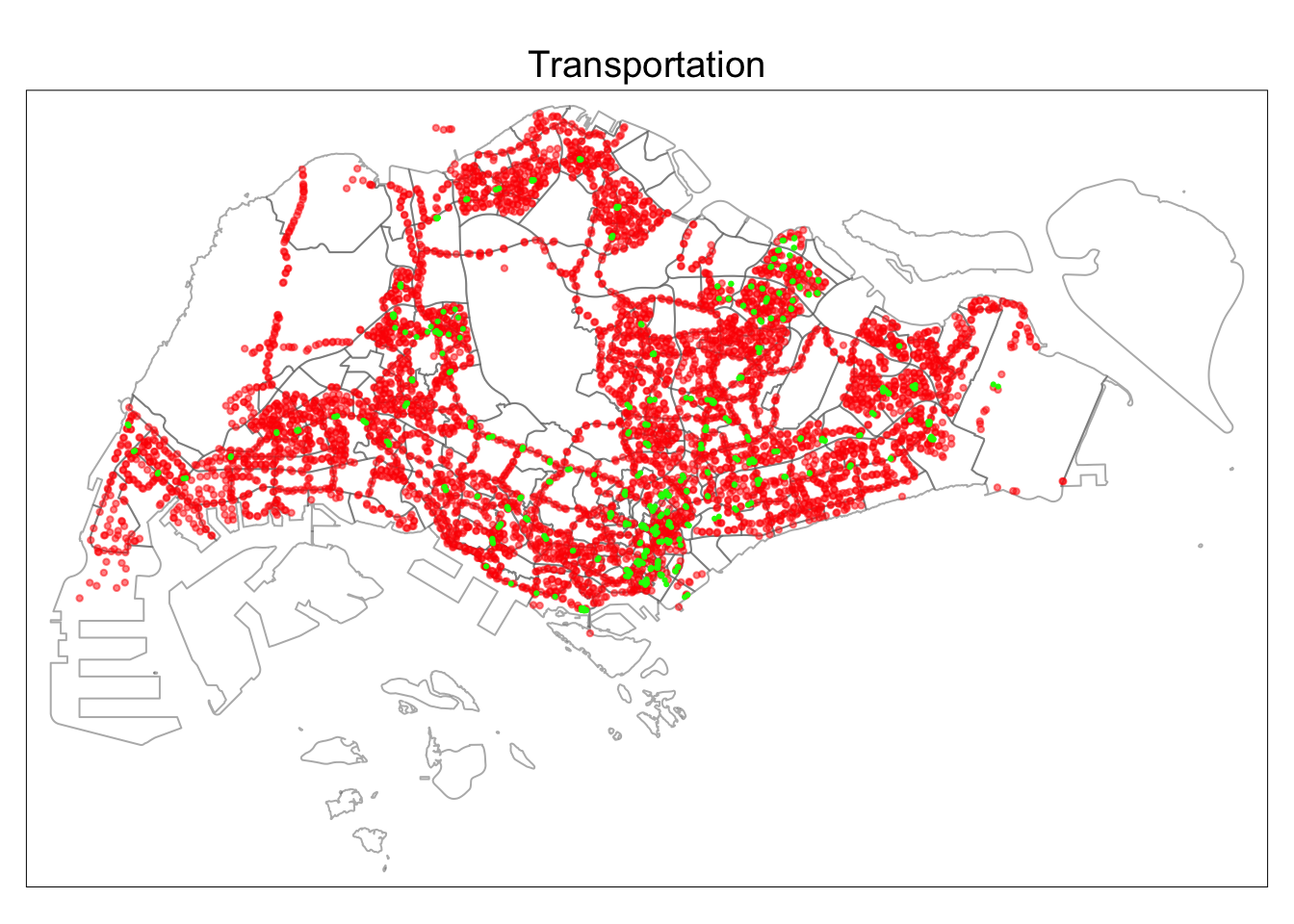
#education
tmap_mode("plot")
tmap mode set to plottingtm_shape(mpsz.sf) +
tm_borders(alpha = 0.5) +
tmap_options(check.and.fix = TRUE) +
tm_shape(primarysch.sf) +
tm_dots(col="pink", size=0.05, alpha=0.5) +
tm_shape(goodprimarysch.sf) +
tm_dots(col="red", size=0.05, alpha=1) +
tm_shape(kindergartens.sf) +
tm_dots(col="purple", size=0.05, alpha=0.5) +
tm_shape(childcare.sf) +
tm_dots(col="yellow", size=0.05, alpha=0.2) +
tm_layout(main.title = "Education",
main.title.position = "center",
main.title.size = 1.2,
frame = TRUE)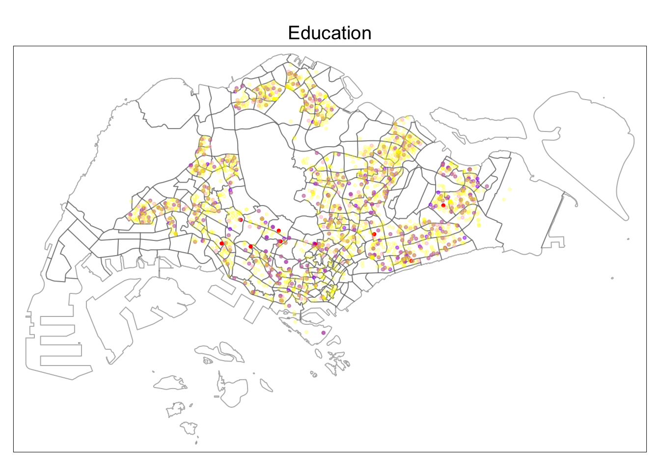
#ammenities
tmap_mode("plot")
tmap mode set to plottingtm_shape(mpsz.sf) +
tm_borders(alpha = 0.5) +
tmap_options(check.and.fix = TRUE) +
tm_shape(parks.sf) +
tm_dots(col="green", size=0.05, alpha=0.5) +
tm_shape(hawkercentre.sf) +
tm_dots(col="blue", size=0.05, alpha=0.5) +
tm_shape(library.sf) +
tm_dots(col="red", size=0.05, alpha=0.5) +
tm_shape(sport.sf) +
tm_dots(col="grey", size=0.05, alpha=0.2) +
tm_shape(shoppingmall.sf) +
tm_dots(col="purple", size=0.05, alpha=0.2) +
tm_shape(supermarket.sf) +
tm_dots(col="brown", size=0.05, alpha=0.2) +
tm_shape(eldercare.sf) +
tm_dots(col="navy", size=0.05, alpha=0.2) +
tm_layout(main.title = "Ammenities",
main.title.position = "center",
main.title.size = 1.2,
frame = TRUE)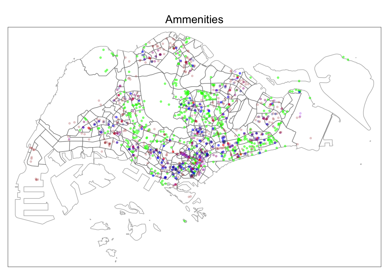
This includes the inherent structural factors of the flats, including Area, Floor Level and Lease Remaining years.
To simplify analysis, we create the an ordinal column for the floor level variable. This code chunk matches the story levels to the list, and gives it an ordinal value based on its relative positioning in the list given (1 would be allocated to “01 TO 03”, 2 allocated to “04 TO 06”….).
# Define the story levels and ordinal values
story_levels <- c("01 TO 03", "04 TO 06", "07 TO 09", "10 TO 12", "13 TO 15", "16 TO 18", "19 TO 21", "22 TO 24", "25 TO 27", "28 TO 30", "31 TO 33", "34 TO 36", "37 TO 39", "40 TO 42", "43 TO 45", "46 TO 48", "49 TO 51")
story_ordinal <- seq_along(story_levels)  # Create the ordinal variable based on the story column
resale$Story_Ordinal <- story_ordinal[match(resale$storey_range, story_levels)]  # Set the labels for the ordinal variable
levels(resale$Story_Ordinal) <- story_levels

# Lastly, we mutate the ordinal variable as a numeric
resale<- resale |>
mutate(Story_Ordinal=as.numeric(Story_Ordinal))The code chunk below seeks to convert the remaining lease period to in terms of years.
str_list <- str_split(resale$remaining_lease, " ")

for (i in 1:length(str_list)) {
  if (length(unlist(str_list[i])) > 2) {
      year <- as.numeric(unlist(str_list[i])[1])
      month <- as.numeric(unlist(str_list[i])[3])
      resale$remaining_lease[i] <- year + round(month/12, 2)
  }
  else {
    year <- as.numeric(unlist(str_list[i])[1])
    resale$remaining_lease[i] <- year
  }
}This includes factors that concern location of amenities to the flat in question. For instance, Proximity to CBD or number of primary schools withi 350 m from the flat in question.
We need to factor in the proximity to CBD in the downtown core. As such let’s take the coordinates of Downtown Core to be the coordinates of the CBD
lat <- 1.287953
lng <- 103.851784

cbd.sf <- data.frame(lat, lng) %>%
  st_as_sf(coords = c("lng", "lat"), crs=4326) %>%
st_transform(crs=3414)resale.sf <- st_as_sf(resale,
coords = c("LONGITUDE",
"LATITUDE"),
crs=4326) %>%
#afterwards, we transform it to SVY21, our desired CRS
st_transform(crs = 3414)One of the things we need to find is the proximity to particular facilities - which we can compute with st_distance(), and find the closest facility (shortest distance) with the rowMins() function of our matrixStats package. The values will be appended to the data frame as a new column.
library(units)
library(matrixStats)
proximity <- function(df1, df2, varname) {
  dist_matrix <- st_distance(df1, df2) |>
    drop_units()
  df1[,varname] <- rowMins(dist_matrix)
  return(df1)
}resale.sf <-
proximity(resale.sf, cbd.sf, "PROX_CBD")
resale.sf <-
proximity(resale.sf, eldercare.sf, "PROX_ELDERCARE")
resale.sf <-
proximity(resale.sf, hawkercentre.sf, "PROX_HAWKERCENTRE")
resale.sf <-
proximity(resale.sf, childcare.sf, "PROX_CHILDCARE")
resale.sf <-
proximity(resale.sf, kindergartens.sf, "PROX_KINDERGARTEN")
resale.sf <-
proximity(resale.sf, parks.sf, "PROX_PARK")
resale.sf <-
proximity(resale.sf, library.sf, "PROX_LIBRARY")
resale.sf <-
proximity(resale.sf, sport.sf, "PROX_SPORT")
resale.sf <-
proximity(resale.sf, busstop.sf, "PROX_BUSSTOP")
resale.sf <-
proximity(resale.sf, shoppingmall.sf, "PROX_SHOPPINGMALL")
resale.sf <-
proximity(resale.sf, supermarket.sf, "PROX_SUPERMARKET")
resale.sf <-
proximity(resale.sf, primarysch.sf, "PROX_PRIMARYSCH")
resale.sf <-
proximity(resale.sf, goodprimarysch.sf, "PROX_GOODPRIMARYSCH")
resale.sf <-
proximity(resale.sf, mrt.sf, "PROX_MRT")Besides proximity, which calculates the shortest distance, we also want to find the number of facilities within a particular radius.
num_radius <- function(df1, df2, varname, radius) {
  dist_matrix <- st_distance(df1, df2) %>%
    drop_units() %>%
    as.data.frame()
  df1[,varname] <- rowSums(dist_matrix <= radius)
  return(df1)
}resale.sf <-
num_radius(resale.sf, busstop.sf, "NUM_BUSSTOP", 350)
resale.sf <-
num_radius(resale.sf, childcare.sf, "NUM_CHILDCARE", 350)
resale.sf <-
num_radius(resale.sf, kindergartens.sf, "NUM_KINDERGARTEN", 350)
resale.sf <-
num_radius(resale.sf, primarysch.sf, "NUM_PRIMARYSCH", 1000)We are finally done with the inclusion of our prox and num variables 😫. We can now save our rds object into our model file for easy retrieval!
saveRDS(resale.sf, "data/model/resale.sf.rds")resale.sf<-read_rds("data/model/resale.sf.rds")
resale.sf<-resale.sf |>
mutate(LEASE_YRS=as.double(LEASE_YRS))With all our data prepared, we are now ready to look into regressing the data to create our prediction models! In particular, we explored the use of OLS, geographical weighted regression, random forest and geographical random forest in this section. 🌳🌲🌴
In order to avoid issues of multicollinearity in regression models, we first visualise our data using a correlation matrix.
resale_nogeo <- resale.sf |>
  st_drop_geometry() |>
  select_if(is.numeric) |>
  select(-PRICE)
corrplot::corrplot(cor(resale_nogeo),
                   diag = FALSE,
                   order = "AOE",
                   tl.pos = "td",
                   tl.cex = 0.5,
                   method = "number",
                   type = "upper")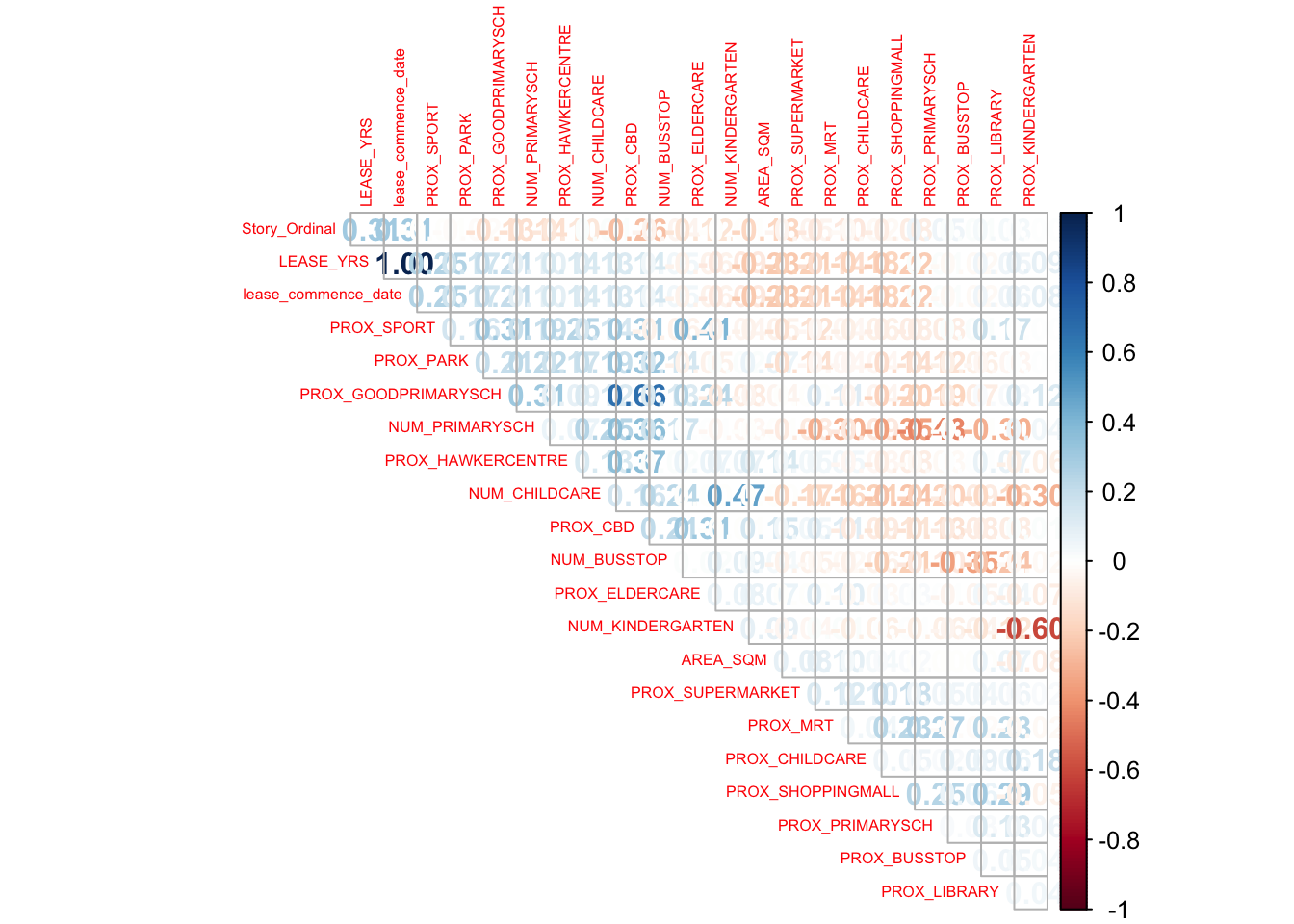
We realise that the variables “lease_commence_date” which is the beginning year of lease, and “LEASE_YRS” which is the number of years left in the lease, are perfectly collinear with a correlation coeffecient of 1. We choose to drop “lease_commence_date” to avoid the problem of perfect collinearity. This creates our final resale df (“resale_final”).
resale_final <- resale.sf |>
select(-lease_commence_date)From the assignment brief, our training data consists of transactions that occurred from 1st January 2021 to 31st December 2022, while test data occurred from January and February 2023.
train_data<-resale_final |>
  filter(month >= "2021-01" & month <= "2022-12")

test_data<-resale_final |>
filter(month >= "2023-01" & month <= "2023-02")First we explored the creation of an OLS model in the code chunk below:
price_mlr<- lm(PRICE~ Story_Ordinal + LEASE_YRS + AREA_SQM + PROX_CBD + PROX_ELDERCARE + PROX_HAWKERCENTRE + PROX_PARK + PROX_LIBRARY + PROX_SPORT + PROX_BUSSTOP + PROX_SHOPPINGMALL + PROX_SUPERMARKET + PROX_GOODPRIMARYSCH + PROX_MRT + NUM_CHILDCARE + NUM_KINDERGARTEN + NUM_PRIMARYSCH, data=train_data)
#removed flat type given that we only consider 4 room flats
#remove geographical variables given GWR
#removed month <- questionable interpretability of coefficient (if generated)

summary(price_mlr)

# saving the result as an rds object
write_rds(price_mlr, "data/model/price_mlr.rds")
We can read the output below
price_mlr_summary<-read_rds("data/model/price_mlr.rds")
price_mlr_summary
Call:
lm(formula = PRICE ~ Story_Ordinal + LEASE_YRS + AREA_SQM + PROX_CBD +
    PROX_ELDERCARE + PROX_HAWKERCENTRE + PROX_PARK + PROX_LIBRARY +
    PROX_SPORT + PROX_BUSSTOP + PROX_SHOPPINGMALL + PROX_SUPERMARKET +
    PROX_GOODPRIMARYSCH + PROX_MRT + NUM_CHILDCARE + NUM_KINDERGARTEN +
    NUM_PRIMARYSCH, data = train_data)

Coefficients:
        (Intercept)        Story_Ordinal            LEASE_YRS
          8.701e+04            1.606e+04            4.435e+03
           AREA_SQM             PROX_CBD       PROX_ELDERCARE
          3.552e+03           -1.631e+01           -8.064e+00
  PROX_HAWKERCENTRE            PROX_PARK         PROX_LIBRARY
         -2.115e+01            6.458e+00           -2.693e+01
         PROX_SPORT         PROX_BUSSTOP    PROX_SHOPPINGMALL
          2.054e+00           -1.732e+01           -1.261e+01
   PROX_SUPERMARKET  PROX_GOODPRIMARYSCH             PROX_MRT
          1.088e+01           -3.043e-01           -1.519e+01
      NUM_CHILDCARE     NUM_KINDERGARTEN       NUM_PRIMARYSCH
-2.821e+03 7.866e+03 -1.098e+04 # a more elegant way of visualising the summary table can be done through using the gtsummary package!
price_mlr<-read_rds("data/model/price_mlr.rds")
gtsummary::tbl_regression(price_mlr)| Characteristic | Beta | 95% CI1 | p-value |
|---|---|---|---|
| Story_Ordinal | 16,063 | 15,624, 16,502 | <0.001 |
| LEASE_YRS | 4,435 | 4,359, 4,510 | <0.001 |
| AREA_SQM | 3,552 | 3,417, 3,688 | <0.001 |
| PROX_CBD | -16 | -17, -16 | <0.001 |
| PROX_ELDERCARE | -8.1 | -9.8, -6.4 | <0.001 |
| PROX_HAWKERCENTRE | -21 | -23, -19 | <0.001 |
| PROX_PARK | 6.5 | 4.2, 8.7 | <0.001 |
| PROX_LIBRARY | -27 | -29, -25 | <0.001 |
| PROX_SPORT | 2.1 | 0.67, 3.4 | 0.004 |
| PROX_BUSSTOP | -17 | -33, -1.5 | 0.031 |
| PROX_SHOPPINGMALL | -13 | -15, -9.9 | <0.001 |
| PROX_SUPERMARKET | 11 | 4.8, 17 | <0.001 |
| PROX_GOODPRIMARYSCH | -0.30 | -0.69, 0.08 | 0.12 |
| PROX_MRT | -15 | -18, -13 | <0.001 |
| NUM_CHILDCARE | -2,821 | -3,295, -2,348 | <0.001 |
| NUM_KINDERGARTEN | 7,866 | 6,864, 8,869 | <0.001 |
| NUM_PRIMARYSCH | -10,982 | -11,670, -10,294 | <0.001 |
| 1 CI = Confidence Interval | |||
gwr method will be used to calibrate a model to predict the HDB resale prices.
We first need to convert the sf data.frame to a SpatialPointDataFrame
train_data_sp<- sf::as_Spatial(train_data)
train_data_sp
class : SpatialPointsDataFrame
features : 23656
extent : 11519.79, 42645.18, 28217.39, 48741.06 (xmin, xmax, ymin, ymax)
crs : +proj=tmerc +lat_0=1.36666666666667 +lon_0=103.833333333333 +k=1 +x_0=28001.642 +y_0=38744.572 +ellps=WGS84 +towgs84=0,0,0,0,0,0,0 +units=m +no_defs
variables : 29
names : PRICE, month, town, flat_type, block, street_name, storey_range, AREA_SQM, flat_model, LEASE_YRS, Story_Ordinal, PROX_CBD, PROX_ELDERCARE, PROX_HAWKERCENTRE, PROX_CHILDCARE, ...
min values : 250000, 2021-01, ANG MO KIO, 4 ROOM, 1, ADMIRALTY DR, 01 TO 03, 70, Adjoined flat, 44.5, 1, 999.393538715878, 1.9938461723793e-05, 30.6031805185926, 1.4128908036435e-05, ...
max values : 1370000, 2022-12, YISHUN, 4 ROOM, 9B, YUNG SHENG RD, 49 TO 51, 145, Type S1, 97.33, 17, 19650.0691667807, 3301.63731683139, 2867.63031236184, 547.386819517238, ... Next, bw.gwr() of GWmodel package will be used to determine the optimal bandwidth to be used.
bw_adaptive <- bw.gwr(PRICE~ Story_Ordinal + LEASE_YRS + AREA_SQM + PROX_CBD + PROX_ELDERCARE + PROX_HAWKERCENTRE + PROX_PARK + PROX_LIBRARY + PROX_SPORT + PROX_BUSSTOP + PROX_SHOPPINGMALL + PROX_SUPERMARKET + PROX_GOODPRIMARYSCH + PROX_MRT + NUM_CHILDCARE + NUM_KINDERGARTEN + NUM_PRIMARYSCH,
                  data=train_data_sp,
                  approach="CV",
                  kernel="gaussian",
                  adaptive=TRUE,
                  longlat=FALSE)

# saving the result as an rds object
write_rds(bw_adaptive, "data/model/bw_adaptive.rds")
The code below can be used to display the model output.
bw_adaptive <- read_rds("data/model/bw_adaptive.rds")Forming model
gwr_adaptive <- gwr.basic(formula = PRICE~ Story_Ordinal + LEASE_YRS + AREA_SQM + PROX_CBD + PROX_ELDERCARE + PROX_HAWKERCENTRE + PROX_PARK + PROX_LIBRARY + PROX_SPORT + PROX_BUSSTOP + PROX_SHOPPINGMALL + PROX_SUPERMARKET + PROX_GOODPRIMARYSCH + PROX_MRT + NUM_CHILDCARE + NUM_KINDERGARTEN + NUM_PRIMARYSCH,
                          data=train_data_sp,
                          bw=bw_adaptive,
                          kernel = 'gaussian',
                          adaptive=TRUE,
                          longlat = FALSE)

# saving the result as an rds object
write_rds(gwr_adaptive, "data/model/gwr_adaptive.rds")
The code below can be used to display the model output.
gwr_adaptive <- read_rds("data/model/gwr_adaptive.rds")The code chunk below extracts the x, y coordinates of the full training and test data sets.
coords<-st_coordinates(resale_final)
coords_train<-st_coordinates(train_data)
coords_test<-st_coordinates(test_data)
Save into rds
write_rds(coords_train, "data/model/coords_train.rds")
write_rds(coords_test, "data/model/coords_test.rds")
Read RDS
coords_train<-read_rds("data/model/coords_train.rds")
coords_test<-read_rds("data/model/coords_test.rds")Drop geometry column of the sf dataframe by using st_drop_geometry()
train_data<-train_data |>
  st_drop_geometry()

write_rds(train_data, "data/model/train_data.rds")
Read RDS
train_data<-read_rds("data/model/train_data.rds")In this section, we will to calibrate a model to predict HDB resale price by using random forest function of ranger package. 🌳🌲🌴🌳🌲🌴
set.seed(1234)
rf<- ranger(PRICE~ Story_Ordinal + LEASE_YRS + AREA_SQM + PROX_CBD + PROX_ELDERCARE + PROX_HAWKERCENTRE + PROX_PARK + PROX_LIBRARY + PROX_SPORT + PROX_BUSSTOP + PROX_SHOPPINGMALL + PROX_SUPERMARKET + PROX_GOODPRIMARYSCH + PROX_MRT + NUM_CHILDCARE + NUM_KINDERGARTEN + NUM_PRIMARYSCH, data=train_data)

summary(rf)

# saving the result as an rds object
write_rds(rf, "data/model/rf.rds")
read RDS object
rf<-read_rds("data/model/rf.rds")
print(rf)
Ranger result
Call:
ranger(PRICE ~ Story_Ordinal + LEASE_YRS + AREA_SQM + PROX_CBD + PROX_ELDERCARE + PROX_HAWKERCENTRE + PROX_PARK + PROX_LIBRARY + PROX_SPORT + PROX_BUSSTOP + PROX_SHOPPINGMALL + PROX_SUPERMARKET + PROX_GOODPRIMARYSCH + PROX_MRT + NUM_CHILDCARE + NUM_KINDERGARTEN + NUM_PRIMARYSCH, data = train_data)
Type: Regression
Number of trees: 500
Sample size: 23656
Number of independent variables: 17
Mtry: 4
Target node size: 5
Variable importance mode: none
Splitrule: variance
OOB prediction error (MSE): 1051737948
R squared (OOB): 0.9372898 Minimise trees to trees=50 for ease of computation.
# determining bandwidth for model
bw_grf_adaptive<-grf.bw(formula = PRICE~ Story_Ordinal + LEASE_YRS + AREA_SQM + PROX_CBD + PROX_ELDERCARE + PROX_HAWKERCENTRE + PROX_PARK + PROX_LIBRARY + PROX_SPORT + PROX_BUSSTOP + PROX_SHOPPINGMALL + PROX_SUPERMARKET + PROX_GOODPRIMARYSCH + PROX_MRT + NUM_CHILDCARE + NUM_KINDERGARTEN + NUM_PRIMARYSCH, dataset = train_data, kernel = "adaptive", coords = coords_train, trees=50)
# saving the result as an rds object
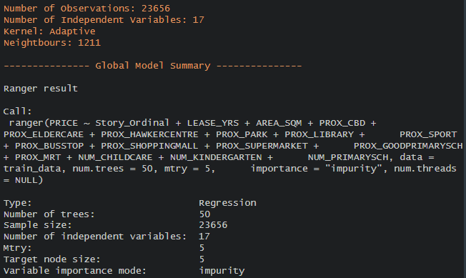
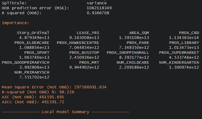
write_rds(bw_grf_adaptive, "data/model/bw_grf_adaptive.rds")we were unable to gain the bandwidth result even after extensive waiting. For the assignment requirements, we will consider the bandwidths generated and choose the one that gives the highest R2 value. The output generated can be seen in the screenshots attached:
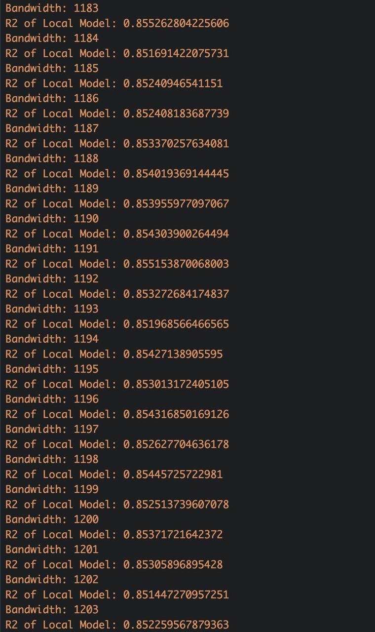
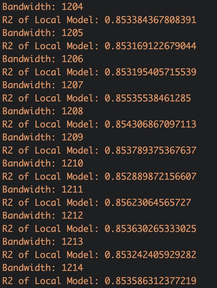
From our data gathered, we find that the optimal bandwidth within the bandwidths calculated is when bandwidth = 1211. We then assign this to the bw_grf_adaptive object
bw_grf_adaptive<-1211set.seed(1234)
gwRF_adaptive<-grf(formula = PRICE~ Story_Ordinal + LEASE_YRS + AREA_SQM + PROX_CBD + PROX_ELDERCARE + PROX_HAWKERCENTRE + PROX_PARK + PROX_LIBRARY + PROX_SPORT + PROX_BUSSTOP + PROX_SHOPPINGMALL + PROX_SUPERMARKET + PROX_GOODPRIMARYSCH + PROX_MRT + NUM_CHILDCARE + NUM_KINDERGARTEN + NUM_PRIMARYSCH,
dframe=train_data,
bw=bw_grf_adaptive, # need to know how to calculate using function
kernel="adaptive",
coords=coords_train,
ntree=50)
# saving the result as an rds object
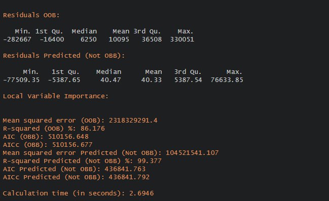
write_rds(gwRF_adaptive, "data/model/gwRF_adaptive.rds")The output rds file generated is 31.7GB, which is larger than what is recommended to push into Git. Therefore, we append screenshots of our outputs instead. 🌳🌲🌴🌳🌲🌴
The code chunk below will be used to combine the test data with the corresponding coordinates data.
test_data <- cbind(test_data, coords_test) %>%
  st_drop_geometry()

write_rds(test_data, "data/model/test_data.rds")Next, predict.grf() of spatialML package will be used to predict the resale value by using the test data and gwRF_adaptive model calibrated earlier.
gwRF_pred <- predict.grf(gwRF_adaptive,
                           test_data,
                           x.var.name="X",
                           y.var.name="Y",
                           local.w=1,
                           global.w=0)

GRF_pred <- write_rds(gwRF_pred, "data/model/GRF_pred.rds")The output of the predict.grf() is a vector of predicted values. It is wiser to convert it into a data frame for further visualisation and analysis.
GRF_pred <- read_rds("data/model/GRF_pred.rds")
GRF_pred_df <- as.data.frame(GRF_pred)
In the code chunk below, cbind() is used to append the predicted values onto test_data.
test_data_p <- cbind(test_data, GRF_pred_df)

#save this as an rds object
write_rds(test_data_p, "data/model/test_data_p.rds")The root mean square error (RMSE) allows us to measure how far predicted values are from observed values in a regression analysis. In the code chunk below, rmse() of Metrics package is used to compute the RMSE.
Metrics::rmse(test_data_p$PRICE,
     test_data_p$GRF_pred)
[1] 44545.08Alternatively, scatterplot can be used to visualise the actual resale price and the predicted resale price by using the code chunk below.
ggplot(data = test_data_p,
       aes(x = GRF_pred,
           y = PRICE)) +
  geom_point()
In the last objective of this take home assignment, a comparison between the conventional OLS method versus the geographically weighted methods should be done.
As this task is focused on predictive modelling, a comparison between the OLS method (a method predominantly for explanatory models) and geographical random forest (for predictive modelling with geographical elements).
| OLS | Geographical random forest | |
|---|---|---|
| Main purpose | Explanatory model for standard regressions | Predictive model for regressions with geographical elements |
| Seeks to minimise | residual sum of squares | mean squared error |
With a basic understanding of how each model works, we hypothesise that the gwRF model will be the most appropriate for analysis, as it accounts for geographical elements included in the resale flat data, as well as the predictive aspect of this model.
To estimate the predictive power of each of the models, we plot each of the predicted values against actual prices in the test data set, and calculate the root MSEs for each of the models.
price_mlr<-read_rds("data/model/price_mlr.rds")
mlr_pred_df<-predict(price_mlr, test_data)
test_data_mlr <- cbind(test_data, mlr_pred_df)

Metrics::rmse(test_data_mlr$PRICE,
     test_data_mlr$mlr_pred_df)
[1] 83524.62ggplot(data = test_data_mlr,
aes(x = mlr_pred_df,
y = PRICE)) +
geom_point()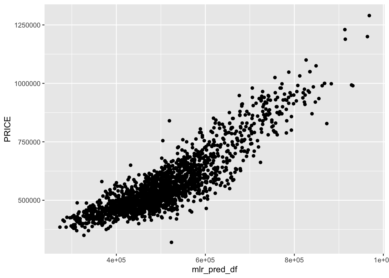
#detailed code chunks can be found in earlier sections
Metrics::rmse(test_data_p$PRICE,
     test_data_p$GRF_pred)
[1] 44545.08ggplot(data = test_data_p,
aes(x = GRF_pred,
y = PRICE)) +
geom_point()
From this comparisons, we conclude that the predictive power of geographical weighted random forest was the most powerful to predict resale prices. this affirms our hypothesis that geographical weighted random forest models are the most appropriate for modelling resale flat data. 🌳🌲🌴
However, our analysis in this assignment was limited🙁:
In the course of this assignment, reference was taken from our senior Megans work. Check out her website here 🤗: https://is415-msty.netlify.app/posts/2021-10-25-take-home-exercise-3/
We also referenced Prof Kam’s in class exercise 9 in this assignment: https://is415-gaa-tskam.netlify.app/in-class_ex/in-class_ex09/in-class_ex09_gwml