In-class Exercise 3: Analytical Mapping

Published

January 16, 2023

1 Installing packages

pacman::p_load(sf, tidyverse, tmap)

Bring data file into R

NGA_wp <- read_rds("data/rds/NGA_wp.rds")

2 Visualising functional water pumps

p1<-tm_shape(NGA_wp) +
  tm_fill("wp_functional",
          n=10,
          style="equal",
          palette="Blues")+
  tm_borders(lwd = 0.1,
             alpha = 1) +
  tm_layout(main.title= "Distribution of functional water point by LGAs", legend.outside = FALSE)

3 Visualising non-functional water pumps

p2<-tm_shape(NGA_wp) +
  tm_fill("total_wp",
          n=10,
          style="equal",
          palette="Blues")+
  tm_borders(lwd = 0.1,
             alpha = 1) +
  tm_layout(main.title= "Distribution of total water point by LGAs", legend.outside = FALSE)

4 Putting the two maps together

tmap_arrange(p2, p1, nrow=1)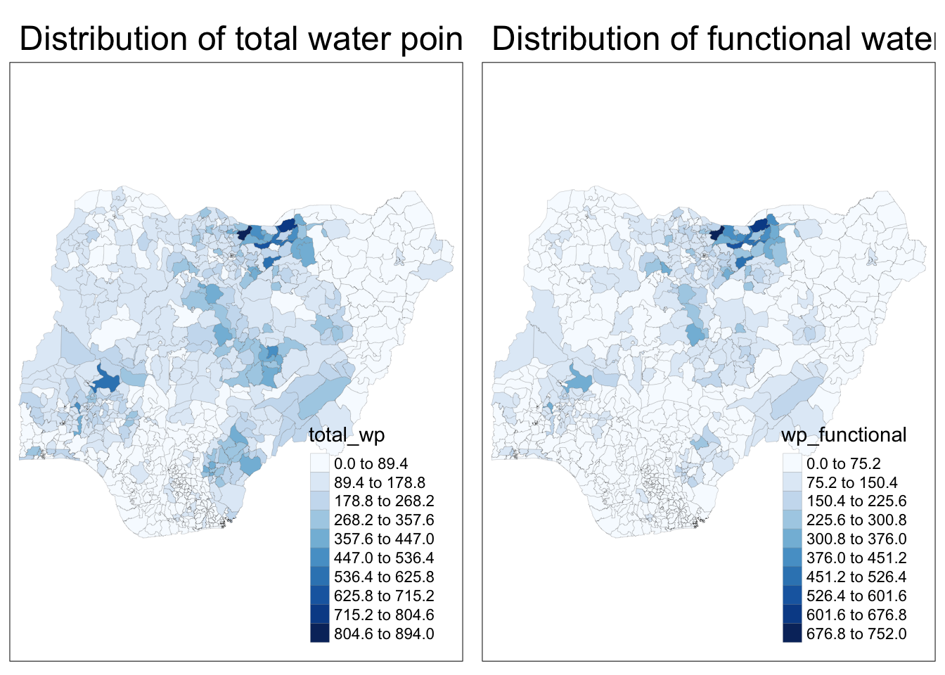

5 Plotting choropleth map for rates

Mapping map rates rather than counts of things.

5.1 Deriving Proportion of Functional Water Points and Non-FUnctional Water Points

NGA_wp <- NGA_wp |> 
  mutate(pct_functional=wp_functional/total_wp) |> 
  mutate(pct_nonfunctional=wp_nonfunctional/total_wp)

5.2 Plotting map of rate

tm_shape(NGA_wp) +
  tm_fill("pct_functional",
          n=10,
          style="equal",
          palette="Blues", 
          legend.hist = TRUE)+
  tm_borders(lwd = 0.1,
             alpha = 1) +
  tm_layout(main.title= "Rate map of functional water point by LGAs", legend.outside = TRUE)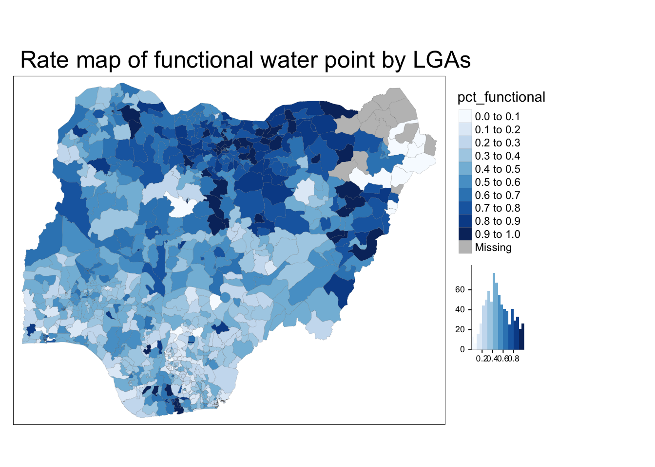

6 Extreme value maps

Extreme value maps are variations of common choropleth maps where the classification is designed to highlight extreme values at the lower and upper end of the scale, identifying outliers.

6.1 Percentile map

special type of quantile map with 6 specific categories: 0-1%,1-10%, 10-50%,50-90%,90-99%, and 99-100%.

6.2 Data preparation

exclude records with NA

NGA_wp <- NGA_wp |> 
  drop_na()

Creating customised classification and extracting values

percent<- c(0, .01, .1, .5, .9, .99,1)
var <- NGA_wp["pct_functional"] |> 
  st_set_geometry(NULL)
quantile(var[,1], percent)

       0%        1%       10%       50%       90%       99%      100% 
0.0000000 0.0000000 0.2169811 0.4791667 0.8611111 1.0000000 1.0000000

Create function to extract variable

# creating a function to do whatever we did above so we can insert different objects to do the same thing
get.var <- function(vname, df) {
  v <- df[vname] %>%
    st_set_geometry(NULL)
    v <- unname(v[,1])
  return(v)
}

Plot function

percentmap <- function(vnam, df, legtitle=NA, mtitle="Percentile Map"){
  percent <- c(0,.01,.1,.5,.9,.99,1)
  var <- get.var(vnam, df)
  bperc <- quantile(var, percent)
  tm_shape(df) +
  tm_polygons() +
  tm_shape(df) +
     tm_fill(vnam,
             title=legtitle,
             breaks=bperc,
             palette="Blues",
          labels=c("< 1%", "1% - 10%", "10% - 50%", "50% - 90%", "90% - 99%", "> 99%"))  +
  tm_borders() +
  tm_layout(main.title = mtitle, 
            title.position = c("right","bottom"))
}

6.3 Test drive the percentile mapping function

percentmap("total_wp", NGA_wp)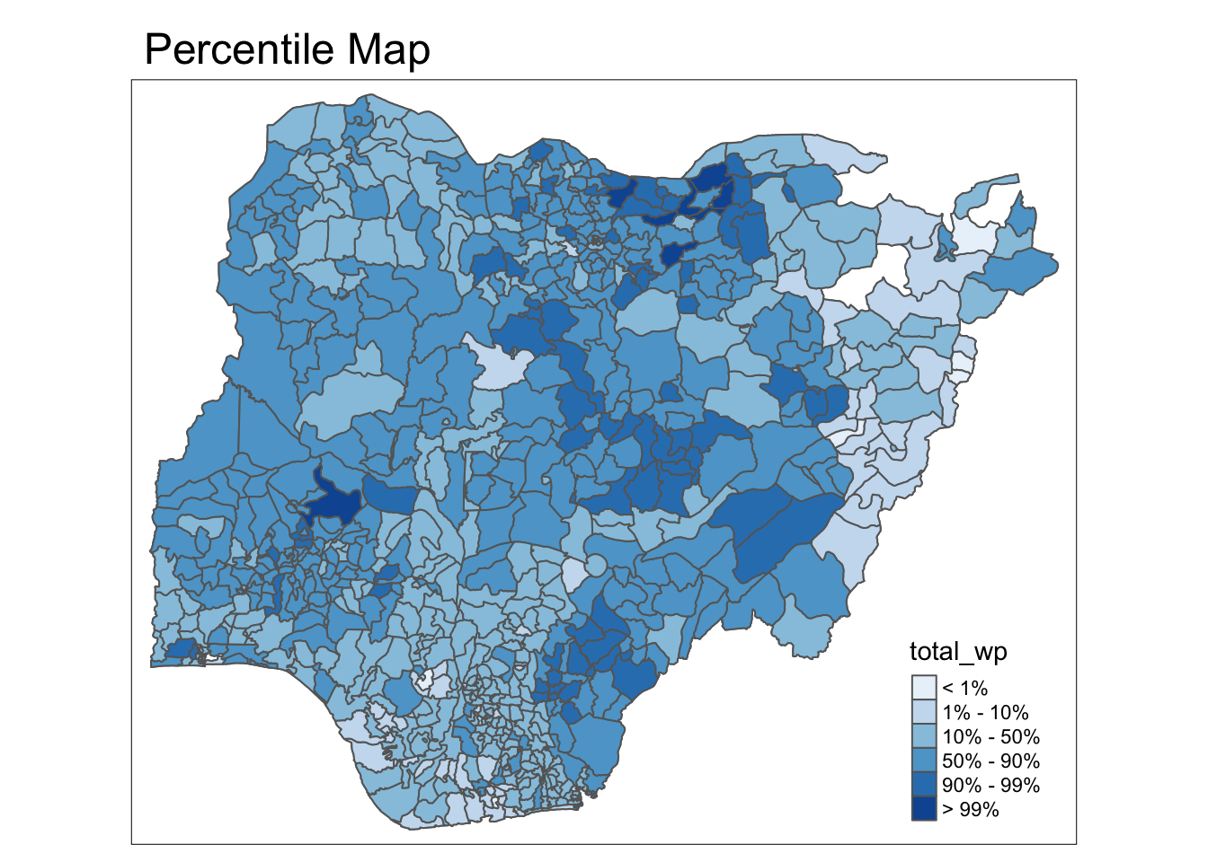

6.4 Box Map

box map is an augmented quartile map, with an additional lower and upper category.

ggplot(data = NGA_wp,
       aes(x = "",
           y = wp_nonfunctional)) +
  geom_boxplot()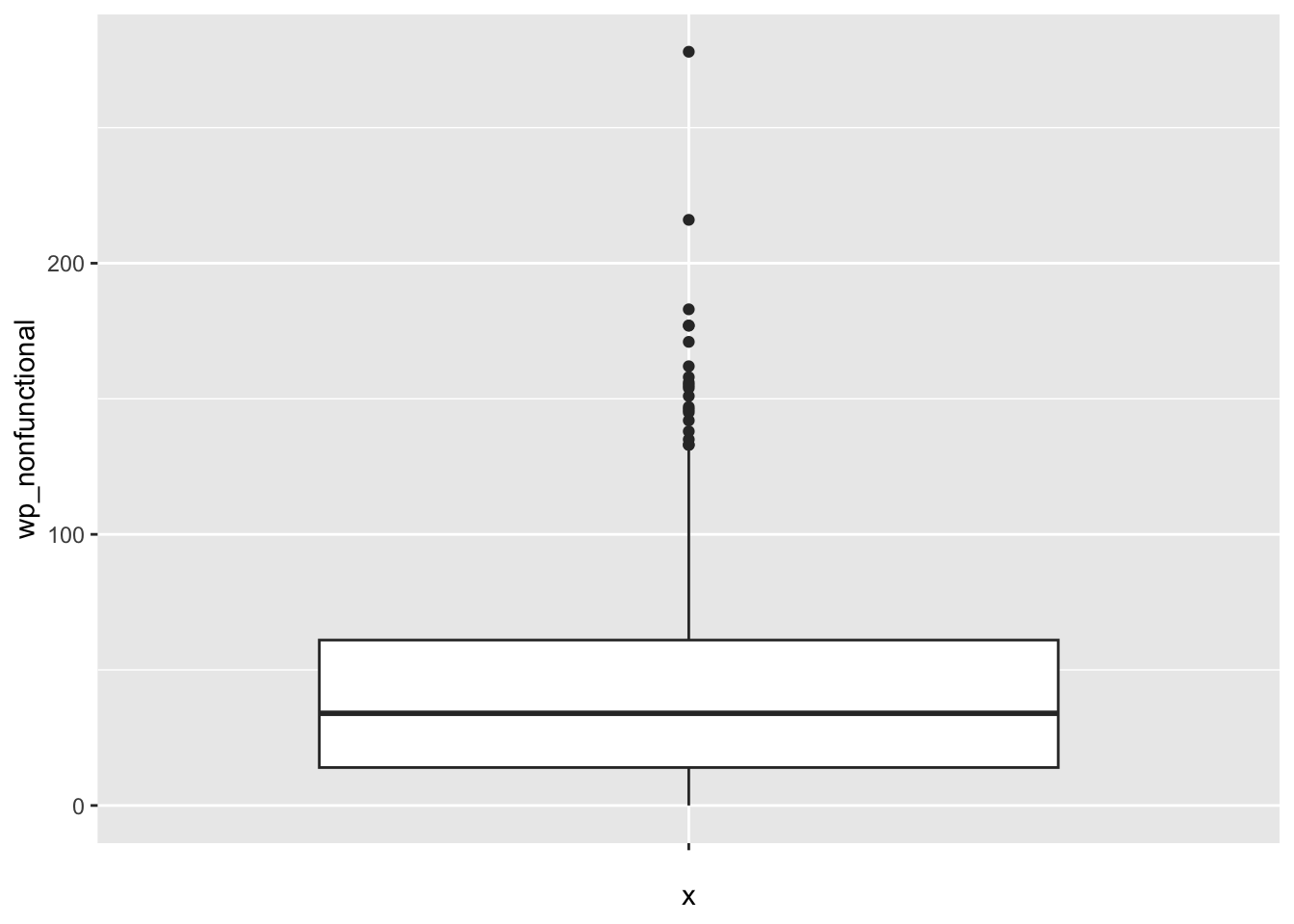

6.4.1 Creating boxbreak function

boxbreaks <- function(v,mult=1.5) {
  qv <- unname(quantile(v))
  iqr <- qv[4] - qv[2]
  upfence <- qv[4] + mult * iqr
  lofence <- qv[2] - mult * iqr
  # initialize break points vector
  bb <- vector(mode="numeric",length=7)
  # logic for lower and upper fences
  if (lofence < qv[1]) {  # no lower outliers
    bb[1] <- lofence
    bb[2] <- floor(qv[1])
  } else {
    bb[2] <- lofence
    bb[1] <- qv[1]
  }
  if (upfence > qv[5]) { # no upper outliers
    bb[7] <- upfence
    bb[6] <- ceiling(qv[5])
  } else {
    bb[6] <- upfence
    bb[7] <- qv[5]
  }
  bb[3:5] <- qv[2:4]
  return(bb)
}

6.5 Creating the get.var function

get.var <- function(vname,df) {
  v <- df[vname] %>% st_set_geometry(NULL)
  v <- unname(v[,1])
  return(v)
}

6.5.1 Test drive the newly created function

var <- get.var("wp_nonfunctional", NGA_wp) 
boxbreaks(var)

[1] -56.5   0.0  14.0  34.0  61.0 131.5 278.0

6.6 Creating boxmap function

boxmap <- function(vnam, df, 
                   legtitle=NA,
                   mtitle="Box Map",
                   mult=1.5){
  var <- get.var(vnam,df)
  bb <- boxbreaks(var)
  tm_shape(df) +
    tm_polygons() +
  tm_shape(df) +
     tm_fill(vnam,title=legtitle,
             breaks=bb,
             palette="Blues",
          labels = c("lower outlier", 
                     "< 25%", 
                     "25% - 50%", 
                     "50% - 75%",
                     "> 75%", 
                     "upper outlier"))  +
  tm_borders() +
  tm_layout(main.title = mtitle, 
            title.position = c("left",
                               "top"))
}

tmap_mode("plot")
boxmap("wp_nonfunctional", NGA_wp)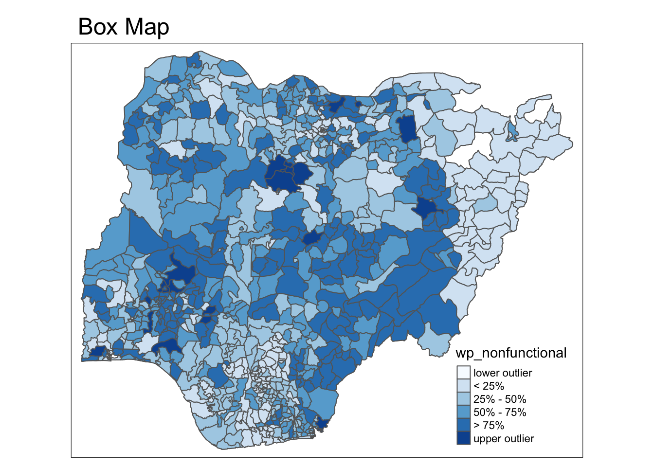

6.7 Recode zero

NGA_wp <- NGA_wp %>%
  mutate(wp_functional = na_if(
    total_wp, total_wp < 0))