pacman::p_load(sf, sfdep, tmap, tidyverse)In-class Exercise 6: Spatial Weights and Applications
1 Installing and loading the R packages
2 The data
For the purpose of this in class exercise, the Hunan data sets will be used. There are two data sets in this use case, they are:
Hunan, a geospatial data set in the ESRI shapefile format, and
Hunan_2012, an attribute dataset in csv format
2.1 Importing geospatial data: shapefile into R environment
The code chunk below uses st_read() of sf package to import Hunan shapefile into R. The imported shapefile will be simple features Object of sf.
hunan <- st_read(dsn = "data/geospatial",
                 layer = "Hunan")
Reading layer `Hunan' from data source
`/Users/pengyouyun/youyunpeng/IS415/In-class_Ex/In-class_Ex06/data/geospatial'
using driver `ESRI Shapefile'
Simple feature collection with 88 features and 7 fields
Geometry type: POLYGON
Dimension: XY
Bounding box: xmin: 108.7831 ymin: 24.6342 xmax: 114.2544 ymax: 30.12812
Geodetic CRS: WGS 842.2 Import csv file into r environment
Next, we will import Hunan_2012.csv into R by using read_csv() of readr package. The output is R dataframe class. Readr will be loaded as part of tidyverse.
hunan2012 <- read_csv("data/aspatial/Hunan_2012.csv")2.3 Combining both data frames using left join
We want the output in an sf dataframe hence, the left dataframe should be hunan, which has a sf format. We need to find a unique identifier, in this case it is by=“County”, where both data frames have a common field.
hunan_GDPPC<-hunan |>
  left_join(hunan2012, by="County") |>
  select(1:4, 7, 15) #selecting only the GDPPC column
2.4 Plotting in a chloropleth map
tmap_mode("plot")
tm_shape(hunan_GDPPC) +
  tm_fill("GDPPC",
          style="quantile",
          palette="Blues",
          totle="GDPPC")+
  tm_borders(alpha = 0.5) +
  tm_layout(main.title= "Distribution of GDP per capita by district",
            main.title.position="center",
            main.title.size=1.2,
            legend.height=0.45,
            legend.width = 0.35,
            frame=TRUE)+
    tm_compass(type="8star", size=2)+
    tm_scale_bar()+
    tm_grid(alpha=0.2)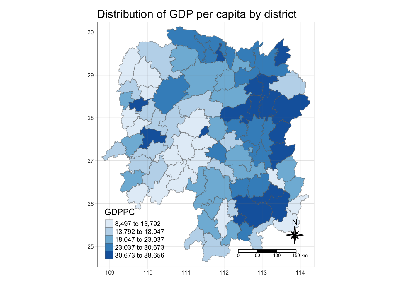
3 Deriving Contiguity Spatial Weights
By and large, there are two types of spatial weights, they are contiguity wights and distance-based weights. In this section, you will learn how to derive contiguity spatial weights by using sfdep.
Two steps are required to derive a contiguity spatial weights, they are:
identifying contiguity neighbour list by
st_contiguity()of sfdep package, andderiving the contiguity spatial weights by using
st_weights()of sfdep package
In this section, we will learn how to derive the contiguity neighbour list and contiguity spatial weights separately. Then, we will learn how to combine both steps into a single process.
3.1 Identifying contiguity neighbours: Queen’s method
In the code chunk below st_contiguity() is used to derive a contiguity neighbour list by using Queen’s method. Note that by default, queen argument is TRUE. Rooks method will be used to identify the first order neighbour if queen=FALSE is used.
nb_queen<-hunan_GDPPC |>
  mutate(nb = st_contiguity(geometry), #creating nearest neighbour list
         .before=1) #put newly created field as the first column

summary(nb_queen$nb) #print the summary of the first lag neighbour list
Neighbour list object:
Number of regions: 88
Number of nonzero links: 448
Percentage nonzero weights: 5.785124
Average number of links: 5.090909
Link number distribution:
1 2 3 4 5 6 7 8 9 11
2 2 12 16 24 14 11 4 2 1
2 least connected regions:
30 65 with 1 link
1 most connected region:
85 with 11 linksnb_queen$County[c(2,3,4,57,85)][1] "Hanshou" "Jinshi" "Li" "Nan" "Taoyuan"This is just the sf version of spdep::poly2nb
3.2 Identifying contiguity neighbours: Rooks’ method
nb_rook<-hunan_GDPPC |>
  mutate(nb = st_contiguity(geometry, #creating nearest neighbour list
         queen=FALSE),
         .before=1) #put newly created field as the first column
Next, we want to Convert neighbour list to distance list
4 Computing contiguity weights
4.1 Contiguity weights: Queen’s method
wm_q <- hunan_GDPPC |>
  mutate(nb = st_contiguity(geometry),
         wt = st_weights(nb),
         .before = 1)
Different from spdep, sfdep can just condense the calculation of contiguity weights into 1 line. Ie we dont have to code the previous chunk under contiguity method.
wt is a standardised weight matrics that is calculated based on 1/no of neighbours in nb list for each observation.
wm_r <- hunan_GDPPC |>
  mutate(nb = st_contiguity(geometry),
         queen = FALSE,
         wt = st_weights(nb),
         .before = 1)
4.2 Identifying higher order neighbours
There are times that we need to identify high order contiguity neighbours. To accomplish the task, st_nb_lag_cumul() should be used as shown in the code chunk below.
nb2_queen <-  hunan_GDPPC %>%
  mutate(nb = st_contiguity(geometry),
         nb2 = st_nb_lag_cumul(nb, 2),
         .before = 1)
Note that if the order is 2, the result contains both 1st and 2nd order neighbors as shown on the print below.
nb2_queenSimple feature collection with 88 features and 8 fields
Geometry type: POLYGON
Dimension: XY
Bounding box: xmin: 108.7831 ymin: 24.6342 xmax: 114.2544 ymax: 30.12812
Geodetic CRS: WGS 84
First 10 features:
nb
1 2, 3, 4, 57, 85
2 1, 57, 58, 78, 85
3 1, 4, 5, 85
4 1, 3, 5, 6
5 3, 4, 6, 85
6 4, 5, 69, 75, 85
7 67, 71, 74, 84
8 9, 46, 47, 56, 78, 80, 86
9 8, 66, 68, 78, 84, 86
10 16, 17, 19, 20, 22, 70, 72, 73
nb2
1 2, 3, 4, 5, 6, 32, 56, 57, 58, 64, 69, 75, 76, 78, 85
2 1, 3, 4, 5, 6, 8, 9, 32, 56, 57, 58, 64, 68, 69, 75, 76, 78, 85
3 1, 2, 4, 5, 6, 32, 56, 57, 69, 75, 78, 85
4 1, 2, 3, 5, 6, 57, 69, 75, 85
5 1, 2, 3, 4, 6, 32, 56, 57, 69, 75, 78, 85
6 1, 2, 3, 4, 5, 32, 53, 55, 56, 57, 69, 75, 78, 85
7 9, 19, 66, 67, 71, 73, 74, 76, 84, 86
8 2, 9, 19, 21, 31, 32, 34, 35, 36, 41, 45, 46, 47, 56, 58, 66, 68, 74, 78, 80, 84, 85, 86
9 2, 7, 8, 19, 21, 35, 46, 47, 56, 58, 66, 67, 68, 74, 76, 78, 80, 84, 85, 86
10 11, 14, 15, 16, 17, 18, 19, 20, 21, 22, 23, 70, 71, 72, 73, 74, 82, 83, 86
NAME_2 ID_3 NAME_3 ENGTYPE_3 County GDPPC
1 Changde 21098 Anxiang County Anxiang 23667
2 Changde 21100 Hanshou County Hanshou 20981
3 Changde 21101 Jinshi County City Jinshi 34592
4 Changde 21102 Li County Li 24473
5 Changde 21103 Linli County Linli 25554
6 Changde 21104 Shimen County Shimen 27137
7 Changsha 21109 Liuyang County City Liuyang 63118
8 Changsha 21110 Ningxiang County Ningxiang 62202
9 Changsha 21111 Wangcheng County Wangcheng 70666
10 Chenzhou 21112 Anren County Anren 12761
geometry
1 POLYGON ((112.0625 29.75523...
2 POLYGON ((112.2288 29.11684...
3 POLYGON ((111.8927 29.6013,...
4 POLYGON ((111.3731 29.94649...
5 POLYGON ((111.6324 29.76288...
6 POLYGON ((110.8825 30.11675...
7 POLYGON ((113.9905 28.5682,...
8 POLYGON ((112.7181 28.38299...
9 POLYGON ((112.7914 28.52688...
10 POLYGON ((113.1757 26.82734...5 Deriving contiguity weights: Queen’s method
Now, you are ready to compute the contiguity weights by using st_weights() of sfdep package.
5.1 Deriving contiguity weights: Queen’s method
In the code chunk below, queen method is used to derive the contiguity weights.
wm_q <- hunan_GDPPC %>%
  mutate(nb = st_contiguity(geometry),
         wt = st_weights(nb,
                         style = "W"),
         .before = 1)
Notice that st_weights() provides tree arguments, they are:
nb: A neighbor list object as created by st_neighbors().
style: Default “W” for row standardized weights. This value can also be “B”, “C”, “U”, “minmax”, and “S”. B is the basic binary coding, W is row standardised (sums over all links to n), C is globally standardised (sums over all links to n), U is equal to C divided by the number of neighbours (sums over all links to unity), while S is the variance-stabilizing coding scheme proposed by Tiefelsdorf et al. 1999, p. 167-168 (sums over all links to n).
allow_zero: If TRUE, assigns zero as lagged value to zone without neighbors.
wm_qSimple feature collection with 88 features and 8 fields
Geometry type: POLYGON
Dimension: XY
Bounding box: xmin: 108.7831 ymin: 24.6342 xmax: 114.2544 ymax: 30.12812
Geodetic CRS: WGS 84
First 10 features:
nb
1 2, 3, 4, 57, 85
2 1, 57, 58, 78, 85
3 1, 4, 5, 85
4 1, 3, 5, 6
5 3, 4, 6, 85
6 4, 5, 69, 75, 85
7 67, 71, 74, 84
8 9, 46, 47, 56, 78, 80, 86
9 8, 66, 68, 78, 84, 86
10 16, 17, 19, 20, 22, 70, 72, 73
wt
1 0.2, 0.2, 0.2, 0.2, 0.2
2 0.2, 0.2, 0.2, 0.2, 0.2
3 0.25, 0.25, 0.25, 0.25
4 0.25, 0.25, 0.25, 0.25
5 0.25, 0.25, 0.25, 0.25
6 0.2, 0.2, 0.2, 0.2, 0.2
7 0.25, 0.25, 0.25, 0.25
8 0.1428571, 0.1428571, 0.1428571, 0.1428571, 0.1428571, 0.1428571, 0.1428571
9 0.1666667, 0.1666667, 0.1666667, 0.1666667, 0.1666667, 0.1666667
10 0.125, 0.125, 0.125, 0.125, 0.125, 0.125, 0.125, 0.125
NAME_2 ID_3 NAME_3 ENGTYPE_3 County GDPPC
1 Changde 21098 Anxiang County Anxiang 23667
2 Changde 21100 Hanshou County Hanshou 20981
3 Changde 21101 Jinshi County City Jinshi 34592
4 Changde 21102 Li County Li 24473
5 Changde 21103 Linli County Linli 25554
6 Changde 21104 Shimen County Shimen 27137
7 Changsha 21109 Liuyang County City Liuyang 63118
8 Changsha 21110 Ningxiang County Ningxiang 62202
9 Changsha 21111 Wangcheng County Wangcheng 70666
10 Chenzhou 21112 Anren County Anren 12761
geometry
1 POLYGON ((112.0625 29.75523...
2 POLYGON ((112.2288 29.11684...
3 POLYGON ((111.8927 29.6013,...
4 POLYGON ((111.3731 29.94649...
5 POLYGON ((111.6324 29.76288...
6 POLYGON ((110.8825 30.11675...
7 POLYGON ((113.9905 28.5682,...
8 POLYGON ((112.7181 28.38299...
9 POLYGON ((112.7914 28.52688...
10 POLYGON ((113.1757 26.82734...5.2 Deriving contiguity weights: Rooks method
wm_r <- hunan %>%
  mutate(nb = st_contiguity(geometry,
                            queen = FALSE),
         wt = st_weights(nb),
         .before = 1)
6 Distance-based weights
There are three popularly used distance-based spatial weights, they are:
fixed distance weights,
adaptive distance weights, and
inverse distance weights (IDW).
6.1 Deriving fixed distance weights
Before we can derive the fixed distance weights, we need to determine the upper limit for distance band by using the steps below:
st_nb_dists()of sfdep is used to calculate the nearest neighbour distance. The output is a list of distances for each observation’s neighbors list.unlist()of Base R is then used to return the output as a vector so that the summary statistics of the nearest neighbour distances can be derived.
geo <- sf::st_geometry(hunan_GDPPC)
nb <- st_knn(geo, longlat = TRUE)
dists <- unlist(st_nb_dists(geo, nb))
Now, we will go ahead to derive summary statistics of the nearest neighbour distances vector (i.e. dists) by usign the coced chunk below.
summary(dists) Min. 1st Qu. Median Mean 3rd Qu. Max.
21.56 29.11 36.89 37.34 43.21 65.80 The summary statistics report above shows that the maximum nearest neighbour distance is 65.80km. By using a threshold value of 66km will ensure that each area will have at least one neighbour.
Now we will go ahead to compute the fixed distance weights by using the code chunk below.
st_dists_band()of sfdep is used to identify neighbors based on a distance band (i.e. 66km). The output is a list of neighbours (i.e. nb).st_weights()is then used to calculate polygon spatial weights of the nb list. Note that:the default
styleargument is set to “W” for row standardized weights, andthe default
allow_zerois set to TRUE, assigns zero as lagged value to zone without neighbors.
wm_fd <- hunan_GDPPC %>%
  mutate(nb = st_dist_band(geometry,
                           upper = 66),
               wt = st_weights(nb),
               .before = 1)
7 Deriving adaptive distance weights
st_knn()of sfdep is used to identify neighbors based on k (i.e. k = 8 indicates the nearest eight neighbours). The output is a list of neighbours (i.e. nb).st_weights()is then used to calculate polygon spatial weights of the nb list. Note that:the default
styleargument is set to “W” for row standardized weights, andthe default
allow_zerois set to TRUE, assigns zero as lagged value to zone without neighbors.
wm_ad <- hunan_GDPPC %>%
  mutate(nb = st_knn(geometry,
                     k=8),
         wt = st_weights(nb),
               .before = 1)
8 Calculate inverse distance weights
In this section, you will derive an inverse distance weights by using the code chunk below.
st_contiguity()of sfdep is used to identify the neighbours by using contiguity criteria. The output is a list of neighbours (i.e. nb).st_inverse_distance()is then used to calculate inverse distance weights of neighbours on the nb list.
wm_idw <- hunan_GDPPC %>%
  mutate(nb = st_contiguity(geometry),
         wts = st_inverse_distance(nb, geometry,
                                   scale = 1,
                                   alpha = 1),
         .before = 1)